Ablation Study of the Bayesian GAN
Although transformers have been dominating the generative AI domain, but I still find this ablation study of Bayesian GAN quite insightful, so I am going to publish it on my website. It is a old project done by: Nicolas Aziere, Mohamad H. Danesh, and Saeed Khorram.
Abstract
This work is about exploring the capacity and limitation of the Bayesian GAN algorithm. The existing framework of the Bayesian GAN is still an unexplored method of learning generative adversarial networks in a bayesian context where the key idea to marginalize the posterior over the weights of the generator and discriminator using a variant of the stochastic gradient descent algorithm namely Hamiltonian Monte-Carlo. It has been demonstrated that this method gives state-of-the-art results in semi-supervised and unsupervised settings and is relatively robust against mode-collapsing. Firstly, we evaluated the influence of some parameters of the algorithm that were not considered in the ablation study of the original paper, and secondly, we trained a Bayesian GAN on a more challenging dataset containing a much larger number of modes that the ones previously studied. Finally, we provide an analysis of the results that will highlight the limitations of the Bayesian GAN and give directions for future work.
Introduction
Generative Adversarial Network (Goodfellow et al., 2014) is one of the most powerful methods to learn the distribution of complex data such as natural images (Brock et al., 2018), audio (Pascual et al., 2017), and text (Press et al., 2017). GAN comprises two main complex mapping functions (usually neural networks): the Generator \(G\) and the Discriminator \(D\). The generator task is to create a candidate sample given a noise vector sampled from a uniform or normal distribution. On the other hand, the discriminator learns to distinguish between the samples candidates generated by the generator and the real data samples in supervised training settings. This adversarial relationship will guide the generator network to create realistic enough candidates to fool the discriminator network and to ideally learn the true data distribution. However, the training procedure of these networks is notoriously difficult, and it is prone to the typical “mode collapse” problem. As most real-world data distributions are highly complex and multi-modal, the challenge for the generator is to output samples that are highly similar to the real data (high precision) yet diverse (high recall) so that the samples can be generalized over the whole data distribution. Nevertheless, in practice, the generator network learns to output a limited number of good quality candidates (high precision) from only one mode of the data. This unique mode will be exploited by the generator to fool the discriminator constantly. This results in candidates that are virtually the same (low recall). To address these issues, various attempts have been made. One is to directly encourage diversity by improving the objective and replacing the Jensen-Shannon divergence of the original GAN paper with enhanced pseudo-metrics such as f-divergence (Nowozin et al., 2016), \(X^2\)-divergence (Mao et al., 2017), and Wasserstein distance (Arjovsky et al., 2017). Further, another thread of research is to train multiple generators (Tolstikhin et al., 2017; Hoang et al., 2018) instead of only one. This hypothesizes that multiple generators can introduce more learning capacity and model the multi-modal data distribution better as in a na¨ıve case, each generator needs to learn a subset of the data. To further extend these ensemble-of-generators models, benefits from Bayesian learning can be exploited to learn the distribution over the GAN parameters. (Saatci & Wilson, 2017), the paper we are analyzing in our work proposed a probabilistic framework for training GAN under Bayesian inference. Bayesian modelling coupled with GAN will introduce new advantages and properties over the classical GAN methods: by learning the posterior over the GAN parameters rather than estimating it as a point mass centered on a single mode (MAP), different modes of the parameters can be sampled which result in totally different generators and discriminators. Moreover, learning the posterior over generator weights can advance more interpretability as each mode will generate different styles of candidates. To be more concise, by investigating the conditional distribution over the parameters of GAN, the true underlying distribution of the data can be modeled more precisely. By applying different priors to represent the distribution of variables, we investigate the effects of those priors over the Bayesian GAN performances. Also, we investigate the weaknesses and limitations represented in (Saatci & Wilson, 2017). In this work, we first go through the idea of the Bayesian GAN, its contributions, and it weaknesses. Next, in section Effect of the prior, we discuss different aspects of out contribution and experiments. Then, our main contribution which is comparing the effects of different priors will be presented. In the experiments section, the experiments we have done will be introduced along with the results we have gotten. Also we will further investigate the validity of the theory and results presented in the (Saatci & Wilson, 2017) through extensive experiments and analysis. The last section is the conclusion, in which we basically summarize our work and highlight its key points.
Bayesian GAN
As the insights introduced in (Saatci & Wilson, 2017) are integral to our work, in this section, we will delve into more details of this paper. The Bayesian GAN framework was proposed to learn the posterior distribution of the generator weights \(\theta_g\) and discriminator weights \(\theta_d\) instead of optimizing for point estimate (analogous to a single maximum likelihood solution). Further, an approximate inference algorithm called Stochastic Gradient Hamiltonian Monte Carlo (SGHMC) which is a gradient-based MCMC method was used to approximate the marginal distributions of \(\theta_g\) and \(\theta_d\) corresponding to generator and discriminator, respectively. To learn a generative model over the data (estimation \(p_{data}\)) in an adversarial framework (Goodfellow et al., 2014), first, a noise vector \(z\) (dimension-d) is sampled from a uniform or normal distribution (dimension-d). Next, the noise vector is fed into the generator parameterized by \(\theta_g\) to create a candidate sample similar to the actual data. In theory, if the generator has sufficient capacity, for a set of \(\theta_g\) it can estimate the CDF inverse-CDF composition required to map a uniform noise to actual data distribution. In the proposed Bayesian GAN by (Saatci & Wilson, 2017), the distribution \(p(\theta_g)\) is placed over the generator parameters, i.e. a distribution over the target distribution of the data. Then, a batch of samples from the true data distribution and the candidate samples from the generators are presented to the discriminator parameterized by \(\theta_d\) intending to distinguish between samples from the real and generated data. The distribution \(p(\theta_d)\) is also introduced over the parameters of the discriminator which entails infinite various settings. Further, we point to a few prominent properties of a Bayesian GAN paper (Saatci & Wilson, 2017) in the following. The author claimed that for a Bayesian GAN, the model is robust to mode collapse, and minimal intervention is required during training for stability where conventionally, a large amount of effort is required to stabilize the GAN training: feature matching, label smoothing, and mini-batch discrimination (Radford et al., 2015). Moreover, the probabilistic ensemble of models for both generator and discriminators allow having complementary models for data, i.e., various styles corresponding to different modes in the data distribution can be generated. Moreover, (Saatci & Wilson, 2017) pointed out the probabilistic formulation of the inference in Bayesian GAN with respect to the adversarial feedback as well as state-of-the-art predictive accuracy using a dramatically small amount of labeled data (e.g., 1%) in a semi-supervised scheme as more useful properties of the Bayesian approach in training GANs. To update the posterior beliefs in response to the adversarial feedback, the authors directly defined two conditional distributions for generator and discriminator parameters to iteratively update the posterior:
\[p(\theta_g| \textbf{z}, \theta_d) \propto \Big( \prod_{i=1}^{n_g} D(G( \textbf{z}^{(i)} ; \theta_g); \theta_d) \Big) \times p(\theta_g| \alpha_g) \label{eq:con_g}\] \[p(\theta_d| \textbf{z}, \textbf{X}, \theta_g) \propto \prod_{i=1}^{n_d} D(\textbf {x}^{(i)} ; \theta_d) \prod_{i=1}^{n_g}(1-D(G(z^{(i)};\theta_g);\theta_d)) \nonumber \times p(\theta_d|\alpha_d) \label{eq:con_d}\]where the \(p(\theta_g|\alpha_g)\) and \(p(\theta_d|\alpha_d)\) are the priors over the parameters of the generator and discriminator, and \(n_g\) and \(n_d\) represent the number of mini-batch samples for generator and discriminator, respectively. Equation 1 basically suggests that to increase the posterior over the generator parameters \(p(\theta_g|z, \theta_d)\) in the neighborhood where the discriminator outputs high probability for the given generated sample as if is from the true distribution. In equation 2, the posterior \(p(\theta_d|z, X, \theta_g)\) will update according to the classification likelihood for data samples from \(X\) and generated samples \(G(z^i ; \theta_g)\) i.e, increase in the neighborhood where the output probability for real data and generated data mismatches the most. It is worth mentioning that if a vague uniform prior over \(\theta_g\) and \(\theta_d\) is assigned, an iterative estimate of Maximum A Posteriori (MAP) optimization would result in the local point mass optima achieved by classical GAN (Goodfellow et al., 2014). The Bayesian formulation of the generator and discriminator parameters will also provide the option to marginalize the noise samples \(z\) from equations 1 and 2 by simply running a few steps of Monte Carlo and obtaining accurate estimates of \(p(\theta_g|\theta_d)\) and \(p(\theta_d|\theta_g)\) which brings useful practical advantages to enhance both generator and discriminator models. To extend the unsupervised equations stated earlier to the semi-supervised scope, given \(n\) unlabeled observations \({x^i}\), and \(n_s\) labeled data \({(x^{i}_{s} , y^{i}_{s} )}\) with class labels \(y^{i}_{s} \in {1, ..., K}\) equations 1 and 2 should be slightly modified. Instead of outputting a probability form 0 to 1, the discriminator here will output a vector of \(K + 1\) different probabilities representing the probability its input is from any of the \(K\) classes in the actual data as well as one class for identifying whether the sample is from the generator or not.
\[p(\theta_g| \textbf{z}, \theta_d) \propto \Big( \prod_{i=1}^{n_g} \sum_{y=1}^K D(G( \textbf{z}^{(i)} ; \theta_g)=y; \theta_d) \Big) p(\theta_g| \alpha_g) \label{eq:semi_g}\] \[p(\theta_d| \textbf{z}, \textbf{x}, \textbf{y}_s, \theta_g) \propto \prod_{i=1}^{n_d} \sum_{y=1}^K D(\textbf {x}^{(i)} = \textbf{y} ; \theta_d) \nonumber \times \prod_{i=1}^{n_g}(1-D(G(z^{(i)};\theta_g);\theta_d)) \nonumber \times \prod_{i=1}^{n_s} D(\textbf{x}_s^{(i)} = \textbf{y}_s^{(i)}; \theta_d) \times p(\theta_d|\alpha_d) \label{eq:semi_d}\]Here, from the perspective of the generator wants to fool the discriminator so that its samples are from the real \(K\) classes in equation 3. On the other hand, the discriminator wants to correctly label the samples that are from the \(K\) classes as well as differentiating from the real and generator samples in equation 4. Finally, in order to effectively sample from the conditional posteriors of the generator and discriminator stated earlier (for both unsupervised and semi-supervised), the Stochastic Gradient Hamiltonian Monte Carlo (SGHMC) (Chen et al., 2014) is proposed use by the authors. SGHMC is reminiscent of momentum-based SGD with noise where it enables sampling with no more computational complexity that SGD and is known to work well for GANs. As claimed by the authors, SGHMC is a key component of the Bayesian deep learning using noisy estimates of gradients which are guaranteed to mix in with a large number of mini-batches.
Effect of the prior
The Bayesian GAN requires different priors for representing the distribution of different variables. When one is dealing with a generator, the noisy input is generally sampled from a prior represented as a normal distribution \(\mathcal{N}(0,I)\). The goal of a Bayesian GAN is to estimate the posterior distribution of weights of both the generator and the discriminator. Using the Bayesian rule, the posterior distribution can be represented as a product of the likelihood and prior over the weights. As stated earlier, in the semi-supervised setting, the posterior distribution has the following form:
\[p(\theta_g| \textbf{z}, \theta_d) \propto \Big( \prod_{i=1}^{n_g} \sum_{y=1}^K D(G( \textbf{z}^{(i)} ; \theta_g)=y; \theta_d) \Big) p(\theta_g| \alpha_g)\]The effect of the prior \(p(\theta_g|\alpha_g)\) becomes less dominant when more data is added to the likelihood. However, we claim that it is advantageous to use a prior more representative of the ideal distribution in order to approximate the posterior distribution more efficiently. Such as proposed in the work of (Kilcher et al., 2017), using a flexible prior distribution can increase the modeling power of a generative model. In their work, they estimate a prior distribution on the latent variable \(z\) using the data by introducing a generator reversal algorithm. They show that constructing a new prior \(p(z)\) from the data instead of using a standard normal distribution is a better-suited choice for various reasons such as: having a better generative model and better modeling performances of the latent structure, more semantically appropriate output. We use the insight of their technique to approximate the best latent variable prior \(p(z)\), however, finding a better prior on the weights of the networks is a more difficult task. Since we do not have any intuition on the type of distribution the weights should model, we designed a simple test case where we evaluate the effect of the prior on a Bayesian GAN.
Synthetic dataset: We do not have the possibility to use the data since they do not give any information about the prior distribution of the weights or of the latent variable \(\textbf(z)\). To alleviate this problem, we defined an arbitrary weights assignment on a generator that will represent the target model taken from a ground truth distribution \(p^*(\theta_g | \alpha_g)\) , and we do the same with \(p^*\textbf(z))\) . Once a generator is sampled, we draw \(N\) samples from \(p^*\textbf(z)\) and pass them through the target generator. The resulting output for each noisy sample will provide a ground truth sample that will form the new training set. When a new dataset is generated, we can train a Bayesian GAN to model the target distribution. We provide an evaluation of training after different variations of the prior \(p(\textbf(z)\) and \(p(\theta_g| \alpha_g)\).
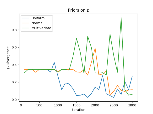
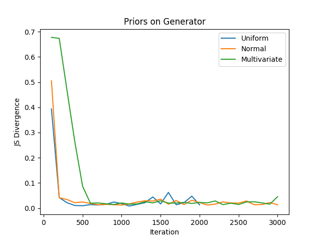
Results: We generated a dataset where \(p^*(\theta_g| \alpha_g)\) and \(p^*\textbf(z))\) follow both a uniform distribution \(Uniform(-1,1)\) . We trained a Bayesian GAN where we varied the prior on \(p^*\textbf(z))\) , the results are shown in Figure 1. We can see that the prior has an influence on the performances, particularly on the convergence speed. However, the stability of the convergence is more stable after a few iterations when a \(Normal(0,1)\) distribution is used as prior. When not much data are seen, the effect of the prior is more dominant, which explains why the $Uniform$ distribution is faster to converge. Oppositely, after a few training iterations, the effect of the prior diminished and the generator can overcome the effect of a bad prior. Figure 2 shows how to change the performance according to the prior distribution set on the generator. The target distribution being uniform, we can see that the convergence speed evolving in the same way as in Figure 1. The effect of the prior is dominant when a few samples are seen and become less dominant over time.
Experiments
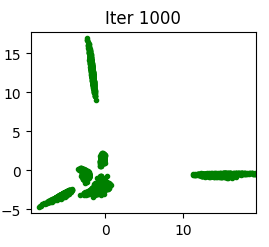
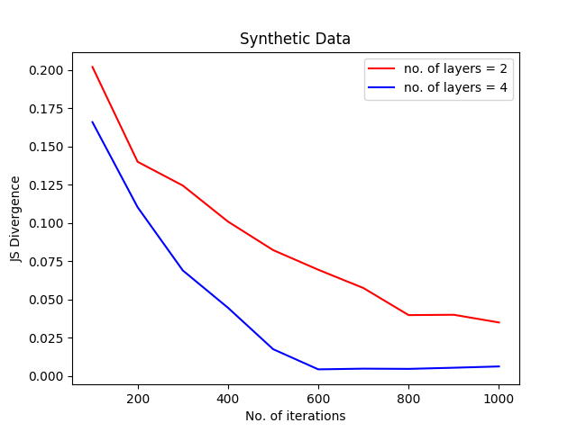
Our experiments were to analyze the limitations (Saatci & Wilson, 2017), which include the number of hidden layers in the generator and discriminator networks, the number of generator and discriminator features, different datasets with more variety in data, and a number of labeled samples. Due to computational limitations (Saatci & Wilson, 2017), the results of experiments on different GAN architectures have not been examined. We have addressed this limitation. According to Figure 3, by just adding two more hidden layers, the generated data distribution is closer to the original data. Also, considering the Jensen-Shannon divergence (Fuglede & Topse, 2004), the Bayesian GAN with more hidden layers showed better convergence.
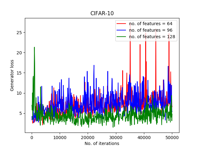
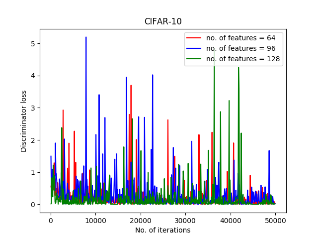
In another experiment, we examined different numbers of features for each of the networks. For this purpose, features of sizes 64, 96, and 128 have been examined. The results of generator loss and discriminator loss are represented in Figure 4.
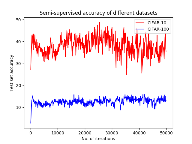
The experiments which were done to investigate the performance of the Bayesian GAN on a new dataset with more variety in data. CIFAR-100 has been used for this purpose. The reason why we chose this dataset is that although it has the same amount of data as CIFAR-10, 50K images for training and 10K images for testing, the number of classes it has is 10 times bigger. This results in having a more diverse dataset with the same amount of data. The results of experimenting on the test set accuracy are drawn in Figure 5. According to Figure 5, it can be inferred that the Bayesian GAN does not perform well in datasets with diversity. This could be due to the priors it uses, which can be addressed in future works.
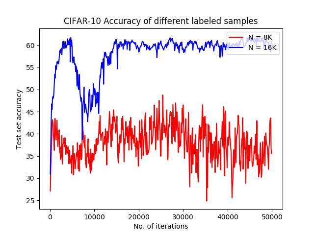
The last experiment we have done is targeting the number of given labeled samples. In this experiment, the CIFAR-10 dataset has been used. The results are depicted in Figure 6. As it was anticipated, the Bayesian GAN got far better accuracy when it had more samples of data.
Discussion
The Bayesian GAN proposed in (Saatci & Wilson, 2017) is valuable in the sense that bridges between Generative Adversarial Networks and Bayesian modeling exploit the best of two worlds. However, we argue there are aspects of the paper that needs further improvement and analysis. One of the most important weaknesses in the paper in our opinion is the choice of prior for both generator and discriminator posterior formulation. In the iterative process of training, the generator distribution only relies on the previous discriminator update which is not desired in cases where the discriminator is not informative in its prediction, i.e., the discriminator tends to assign equal probabilities to all data samples resulting in equal likelihood for all generators (He et al., 2018). Our attempts to alleviate this issue are presented in section Effect of the prior. Further, during experimenting, we faced a few deficiencies. The first one is about experimenting with the different sizes of feature vectors. Standard deviation is not a good measurement to validate the results of the discriminator network loss. Also, due to the huge amount of computations that GANs require. That is why the number of iterations is limited, and datasets with more data have not been experimented with.
On the other hand, to point out one of the key contributions of the Bayesian GAN approach, we believe the use of Stochastic Gradient Hamiltonian Monte Carlo (SGHMC) (Chen et al., 2014) in inference has introduced a novel approach to estimating the posterior since the exact formulation is not practical. Algorithmically, SGHMC is very close to momentum SGD which is inspiring since SGHMC can be used in applications SGD has shown promising performance in recent deep learning breakthroughs and the technical insights of using SGD can be translated to SGHMC for Bayesian approaches. In addition, extensions including Adam-HMC (Kingma & Ba, 2014) etc. can be put into practice.
Conclusion
This paper proposed an ablation study of the Bayesian GAN method containing a set of additional experiments and an analysis of its advantages and limitations. Finding the right architecture and set of parameters for a model is not a trivial task, we found that the number of layers, the feature size, and the priors greatly influence the learning capabilities of the network. We varied the size of the networks and the size of the feature vector in order to understand the previous choices of the original author of the Bayesian GAN method. We proposed a method to evaluate the effect of the priors by introducing a new dataset generator generated by a target model where the target priors are known. Another significant limitation of the model is its poor ability to address a large number of classes in a dataset such as CIFAR-100. There is still a large set of unexplored areas when investigating the theoretical properties of GANs using Bayesian modeling, and we let open these studies for future work.