Generating Gaussian Samples From A Uniform Distribution

Introduction

The rand() function generates uniformly-distributed numbers between 0~RAND_MAX, where RAND_MAX depends on the implementation and language. For example, in Matlab, RAND_MAX is 1, while in C/C++ RAND_MAX is the maximum integer number of the int representation.

The problem is then how to generate numbers distributed with the Gaussian PDF based on rand(), and how to check that what you generate is in fact Gaussian or Pareto distributed. There are many approaches to generate normally-distributed random numbers starting from a uniform distribution. This report describes three methods: Inverse Transform Sampling, Box-Muller Algorithm, and Ziggurat Algorithm. Moreover, finally, we show how our empirically observed data can be verified.

Inverse Transform Sampling

Inverse transform sampling applies the inverse function of the target cumulative distribution function (CDF) to transform a uniform sample into a target-distributed sample. Here, in our case, the target distribution of interest is the normal distribution. The idea behind inverse transform sampling is that for any distribution, the cumulative probability is always uniformly distributed.

As we know, the CDF for normal distribution is defined as: \(CDF(x) = \int_{-\infty}^{x} PDF(t)dt = \int_{-\infty}^{x} \frac{1}{\sqrt{2\pi}} e^{\frac{-t^2}{2}}dt\)

However, the problem is that the above integral does not have a closed-form solution. One approach to address this problem is to measure the CDF of normal distribution using the error function. By definition, the error function is: \(erf(x) = \frac{2}{\sqrt{\pi}}\int_{0}^{x} e^{-t^2}dt\)

By doing a small change of variable: \(t^2 = \frac{z^2}{2}\) within the integration, we will have: \(erf(x) = \frac{2}{\sqrt{2\pi}} \int_{0}^{x\sqrt{2}} e^{\frac{-z^2}{2}}dz = \\ 2( \frac{1}{\sqrt{2\pi}} \int_ {-\infty}^{x\sqrt{2}} e^{\frac{-z^2}{2}}dz - \frac{1}{\sqrt{2\pi}} \int_{-\infty}^{0} e^{\frac{-z^2}{2}}dz )\)

The integrals on the last line are both values of the CDF of the standard normal distribution: \(\Phi (x) = \frac{1}{\sqrt{2\pi}} \int_{-\infty}^{x} e^{\frac{-z^2}{2}}dz\)

Thus: \(erf(x) = 2(\Phi(x\sqrt{2}) - \Phi(0)) = 2\Phi(x\sqrt{2}) - 1\)

This equation offers an advantage and a disadvantage. The disadvantage is that it is not possible to evaluate inverse error function directly. However, the advantage is that the inverse error function can be approximated. One of the most common methods to do so is to approximate using the Taylor series.

The Taylor series approximation of a function around a point requires finding the derivatives of the function at that point. For the inverse erf, we set \(x = 0\) as the point to be approximated around, since the inverse erf and the erf functions are symmetric around \(x=0\): \(erf^{-1}(x) = erf^{-1}(0) +\) \(\frac{erf^{-1^{'}}(0)}{1!}x +\) \(\frac{erf^{-1^{''}}(0)}{2!}x^2 + ...\)

In the first term, we have \(erf^{-1}(0) = 0\). So to approximate the \(erf^{-1}\), we should calculate the rest of the terms of the Taylor series. The derivatives of \(erf^{-1}\) are: \(erf^{-1^{'}}(x) = \frac{\sqrt{\pi}}{2} e^{(erf^{-1}(x))^2}\)
\(erf^{-1^{''}}(x) = \frac{\sqrt{\pi}}{2} e^{(erf^{-1}(x))^2} 2 erf^{-1}(x) erf^{-1^{'}}(x) = (erf^{-1^{'}}(x))^2 2 erf^{-1}(x)\)

When deriving higher derivatives of the \(erf^{-1}\), starting from the second derivative, each derivate of order \(n\) is a product of the first derivative to the power of \(n\), and a polynomial of \(erf^{-1}\). By investigating and simplifying further, we see that all the even-powered terms in the Taylor series have no constant term for their polynomials. Thus, the Taylor series approximation only involves odd-powered terms. That results in the following simplified Taylor series approximation of the \(erf^{-1}(x)\): \(erf^{-1}(x) = \frac{\sqrt{\pi}}{2} (x + \frac{\pi}{12}x^3 + \frac{7\pi}{480}x^5 + ...)\)

Now, the above Taylor approximations of \(erf^{-1}\) can be used to approximate the inverse CDF of standard normal distribution. Clearly, including more terms in the Taylor series result in a better approximation of the true inverse CDF.

Finally, we can now generate normally-distributed samples using inverse transform sampling. To do so, following steps need to be taken:

• Sample a point from a uniform distribution.
• Apply Taylor series approximation of inverse normal CDF.
• Generate normal samples.

In conclusion, this method can generate any random variable if its CDF is easily calculated. If it is not, using this method would be challenging as discussed earlier. It requires one to use complex approximation methods. Other methods such as Box-Muller and rejection sampling could be helpful in that regard.

Box-Muller Algorithm

The Box-Muller method gets two samples from a uniform distribution and generates two independent samples from a standard normal distribution. To do so, consider two sets of random samples (IID) with equal lengths drawn from the \(U(0,1)\), \(u_0\) and \(u_1\). From these two sets, one can generate two sets of normally-distributed random variables, drawn from \(N(\mu=0, \sigma=1)\) which we call \(n_0\) and \(n_1\), where: \(n_0 = \sqrt{-2 \ln(u_0)} \cos(2\pi u_1) \\ n_1 = \sqrt{-2 \ln(u_0)} \sin(2\pi u_1)\)

If we assume to position the variables \(u_0, u_1\) in the Cartesian plane, we can take advantage of the relationship between Cartesian coordinates and polar coordinates \((r, \theta)\), by: \(n_0 = R * \cos{\theta} \\ n_1 = R * \sin{\theta}\)

Now, in the polar coordinates, a bivariate normal distribution \((n_0, n_1)\) has a norm $R$ corresponding to \(\sqrt{-2 \ln u_0}\), and an angle \(\theta\) corresponding to \(2 \pi u_1\). This allows us to map the variables defined in the original Cartesian system to the normally-distributed variables \(n_0, n_1\). By doing so, we will reach the variables defined in the first equation (re \(n_0\)).

Implementation

Implementation of the algorithm can be found here:

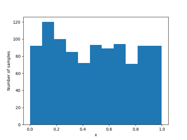
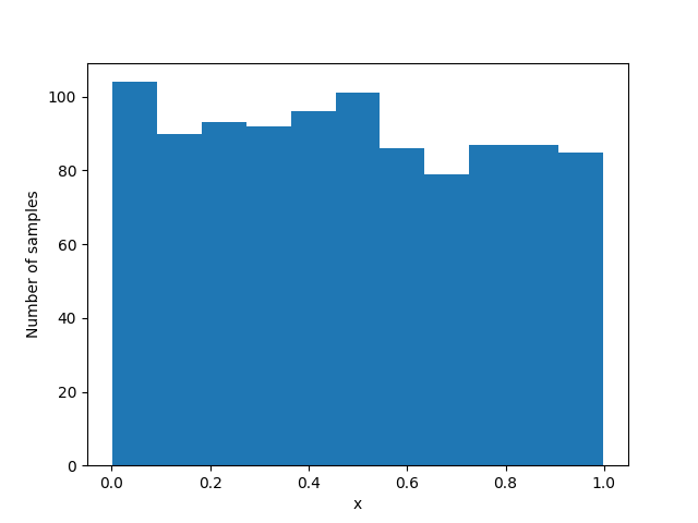
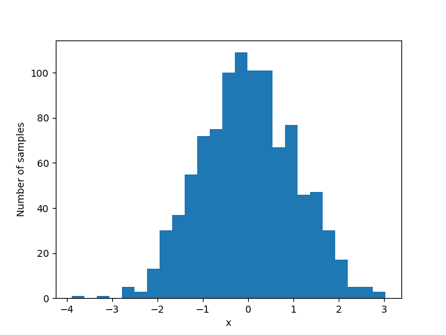
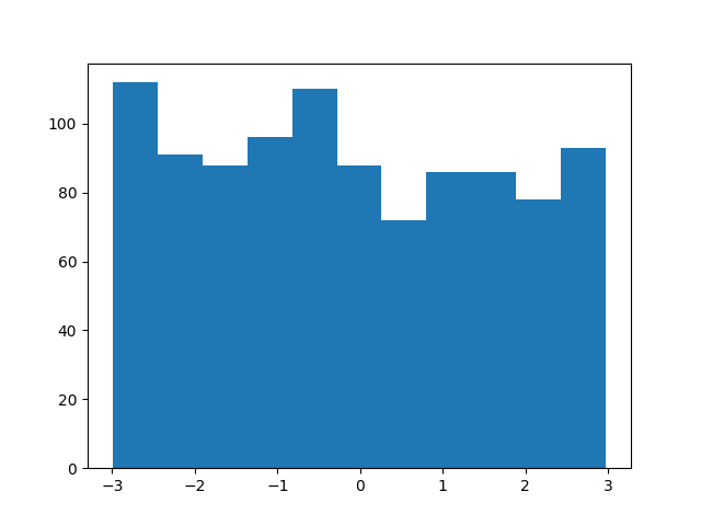
Figure bellow shows the output of an example run of the provided code:

Ziggurat (Rejection Sampling) Algorithm

The idea behind rejection sampling is that if one cannot sample from a distribution (target), another distribution function (proposal) could be used for sampling. However, since the target distribution and the proposal distribution are different, drawn samples (from the proposal distribution) must follow the target distribution. It means that regions with a high probability in the target distribution should be sampled more.

Assume that we have a uniform distribution as the proposal function and a normal distribution as the target function. First, the proposal distribution should encapsulate the target distribution, so that drawn samples could be either rejected or accepted. To do so, the proposal distribution should be scaled with respect to the mean and standard deviation of the target distribution. Then, the proposal PDF is separated into a series of segments with equal areas ( bins). Next, the sampling process begins: a sample is drawn from the scaled proposal distribution. We look it up to see which segment it belongs to. If the corresponding segment density in the proposal function is lower than the corresponding segment density in the target function, the sample is accepted; otherwise, it is rejected. By repetitively doing this, more samples within the acceptable region are taken.

There are issues with the naive rejection sampling method, which the Ziggurat algorithm addresses: first, in the naive rejection sampling method, a large number of samples will be rejected since we have only one segment. Second, by discretizing the proposal PDF using segmentation, we make it computationally tractable to evaluate whether to reject or accept a candidate.

Implementation

Ziggurat implementation is available here:

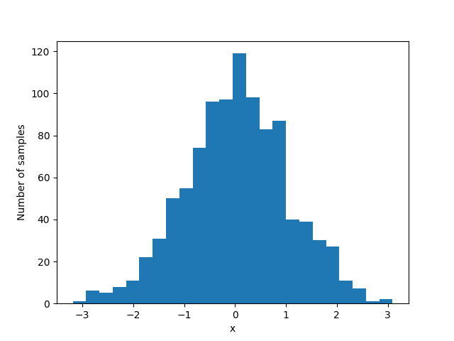
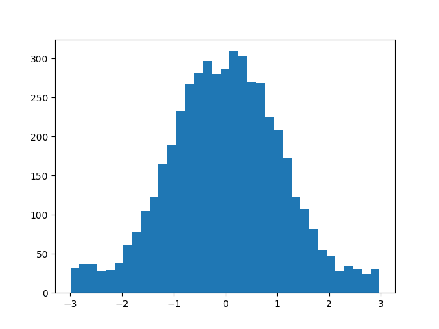
Figure bellow shows an example output of running the code:

Verifying Results

Finally, in order to verify the results, one can use the goodness-of-fit tests. They are statistical approaches aiming to determine whether a set of observed values match those expected under the normal distribution. There are several approaches for the goodness-of-fit tests, including the chi-square, the Kolmogorov-Smirnov test, and the Lilliefors test. The chi-square tests the validity of a claim made about a population of observed values based on a random sample.

The chi-square test requires samples to be represented in a categorical format, which is limiting in our case. As a replacement, one can use the Kolmogorov-Smirnov test for normality, but the mean and the standard deviation must be known beforehand; nevertheless, the Kolmogorov-Smirnov test yields conservative results. The Lilliefors test tackles this problem by giving more accurate results. The only difference between the Lilliefors test and the Kolmogorov-Smirnov test is that the former uses the Lilliefors Test Table while the latter uses the Kolmogorov-Smirnov Table. Otherwise, both have the same calculations.

For the Lilliefors Test, we need to define our null hypothesis and the alternate hypothesis. The null hypothesis ( \(H_0\)) for the test is that the data comes from a normal distribution, and the alternate hypothesis (\(H_1\)) is that the data does not come from a normal distribution.

The calculation steps of Lilliefors test are:

• calculate z-score \(Z_i\) using the following equation:

  \[Z_i = \frac{X_i - \bar{X}}{s}, i = 1, 2, ..., n\]

  where \(Z_i\) is the individual z-scores for every member in the sample set, \(X_i\) is the individual data point, \(\bar{X}\) is the sample mean, and \(s\) is the standard deviation.

• calculate the test statistic, which is the empirical distribution function based on the \(Z_i\)s:

  \[D = \sup_{X} |F_0 (X) - F_{data} (X)|\]

  where \(F_0\) is the the standard normal distribution function (hypothesized distribution), and \(F_{data}\) is the empirical distribution function of the observed values. - find the critical value for the test from the Lilliefors Test table and reject the null hypothesis if the test statistic \(D\) is greater than the critical value.