Summary: Artificial Intelligence - A Modern Approach

1. Introduction

• Definition of intelligence: perceive, understand, predict, and manipulate a world far larger and more complicated than itself.
• AI definition lies in these aspects: “thought processes and reasoning” vs “behaviour” and “humanly” vs “rationally”.
  • Acting humanly: Turing test.
  • Thinking humanly: Cognitive modeling approach, in line with cognitive science.
  • Thinking rationally: The “laws of thought” approach, in line with logic.
  • Acting rationally: The rational agent approach, which is an agent acting so as to achieve the best expected outcome.
• The quest for “artificial flight” succeeded when the Wright brothers and others stopped imitating birds and started using wind tunnels and learning about aerodynamics.
• Aristotle: actions are justified by a logical connection between goals and knowledge of the action’s outcome.
• Craik specified the three key steps of a knowledge-based agent: (1) the stimulus must be translated into an internal representation, (2) the representation is manipulated by cognitive processes to derive new internal representations, and (3) these are in turn retranslated back into action.
• knowledge representation the study of how to put knowledge into a form that a computer can reason with.
• The new back-propagation learning algorithms for multilayer networks that were to cause an enormous resurgence in neural-net research in the late 1980s were actually discovered first in 1969 (Bryson and Ho, 1969).
• AI was founded in part as a rebellion against the limitations of existing fields like control theory and statistics, but now it is embracing those fields.

2. Intelligent Agents

• Agent perceives its environment through sensors and acts upon that environment through actuators. Mathematically speaking, agent’s behavior is described by the agent function that maps any given percept sequence to an action.
• Percept sequence is the complete history of everything the agent has ever perceived.
• The agent function is an abstract mathematical description; the agent program is a concrete implementation, running within some physical system.
• As a general rule, it is better to design performance measures according to what one actually wants in the environment, rather than according to how one thinks the agent should behave.
• What is rational at any given time depends on four things:
  • The performance measure that defines the criterion of success.
  • The agent’s prior knowledge of the environment.
  • The actions that the agent can perform.
  • The agent’s percept sequence to date.
• In designing an agent, the first step must always be to specify the task environment as fully as possible. Task environment consists of Performance, Environment, Actuators, and Sensors.
• Fully observable vs. partially observable. If an agent’s sensors give it access to the complete state of the environment at each point in time, then we say that the task environment is fully observable. A task environment is effectively fully observable if the sensors detect all aspects that are relevant to the choice of action; relevance, in turn, depends on the performance measure. An environment might be partially observable because of noisy and inaccurate sensors or because parts of the state are simply missing from the sensor data.
• Single agent vs. multiagent. We have described how an entity may be viewed as an agent, but we have not explained which entities must be viewed as agents. The key distinction is whether B’s behavior is best described as maximizing a performance measure whose value depends on agent A’s behavior.
• Deterministic vs. stochastic. If the next state of the environment is completely determined by the current state and the action executed by the agent, then we say the environment is deterministic; otherwise, it is stochastic. We say an environment is uncertain if it is not fully observable or not deterministic. One final note: our use of the word “stochastic” generally implies that uncertainty about outcomes is quantified in terms of probabilities; a nondeterministic environment is one in which actions are characterized by their possible outcomes, but no probabilities are attached to them. Nondeterministic environment descriptions are usually associated with performance measures that require the agent to succeed for all possible outcomes of its actions.
• Episodic vs. sequential. In an episodic task environment, the agent’s experience is divided into atomic episodes. In each episode the agent receives a percept and then performs a single action. Crucially, the next episode does not depend on the actions taken in previous episodes. Many classification tasks are episodic. In sequential environments, on the other hand, the current decision could affect all future decisions.
• Static vs. dynamic. If the environment can change while an agent is deliberating, then we say the environment is dynamic for that agent; otherwise, it is static. Static environments are easy to deal with because the agent need not keep looking at the world while it is deciding on an action, nor need it worry about the passage of time. Dynamic environments, on the other hand, are continuously asking the agent what it wants to do; if it hasn’t decided yet, that counts as deciding to do nothing. If the environment itself does not change with the passage of time but the agent’s performance score does, then we say the environment is semidynamic.
• Discrete vs. continuous. The discrete/continuous distinction applies to the state of the environment, to the way time is handled, and to the percepts and actions of the agent.
• Known vs. unknown. Strictly speaking, this distinction refers not to the environment itself but to the agent’s (or designer’s) state of knowledge about the “laws of physics” of the environment. In a known environment, the outcomes (or outcome probabilities if the environment is stochastic) for all actions are given. Obviously, if the environment is unknown, the agent will have to learn how it works in order to make good decisions. Note that the distinction between known and unknown environments is not the same as the one between fully and partially observable environments.
• Simple reflex agents select actions on the basis of the current percept, ignoring the rest of the percept history. Simple reflex agents have the admirable property of being simple, but they turn out to be of limited intelligence. Escape from infinite loops is possible if the agent can randomize its actions.
• Model-based reflex agents. The most effective way to handle partial observability is for the agent to keep track of the part of the world it can’t see now. That is, the agent should maintain some sort of internal state that depends on the percept history and thereby reflects at least some of the unobserved aspects of the current state. Updating this internal state information as time goes by requires two kinds of knowledge to be encoded in the agent program. First, we need some information about how the world evolves independently of the agent. Second, we need some information about how the agent’s own actions affect the world.
• Goal-based agents. Knowing something about the current state of the environment is not always enough to decide what to do. As well as a current state description, the agent needs some sort of goal information that describes situations that are desirable. Notice that decision making of this kind is fundamentally different from the condition– action rules described earlier, in that it involves consideration of the future—both “What will happen if I do such-and-such?” and “Will that make me happy?” In the reflex agent designs, this information is not explicitly represented, because the built-in rules map directly from percepts to actions.
• Utility-based agents. Goals alone are not enough to generate high-quality behavior in most environments. Goals just provide a crude binary distinction between “happy” and “unhappy” states. A more general performance measure should allow a comparison of different world states according to exactly how happy they would make the agent. An agent’s utility function is essentially an internalization of the performance measure. If the internal utility function and the external performance measure are in agreement, then an agent that chooses actions to maximize its utility will be rational according to the external performance measure. In two kinds of cases, goals are inadequate but a utility-based agent can still make rational decisions. First, when there are conflicting goals, only some of which can be achieved, the utility function specifies the appropriate tradeoff. Second, when there are several goals that the agent can aim for, none of which can be achieved with certainty, utility provides a way in which the likelihood of success can be weighed against the importance of the goals.
• Learning agents. A learning agent can be divided into four conceptual components. The most important distinction is between the learning element, which is responsible for making improvements, and the performance element, which is responsible for selecting external actions. The performance element is what we have previously considered to be the entire agent: it takes in percepts and decides on actions. The learning element uses feedback from the critic on how the agent is doing and determines how the performance element should be modified to do better in the future. The critic tells the learning element how well the agent is doing with respect to a fixed performance standard. The critic is necessary because the percepts themselves provide no indication of the agent’s success. Conceptually, one should think of it as being outside the agent altogether because the agent must not modify it to fit its own behavior. The last component of the learning agent is the problem generator. It is responsible for suggesting actions that will lead to new and informative experiences. The point is that if the performance element had its way, it would keep doing the actions that are best, given what it knows. But if the agent is willing to explore a little and do some perhaps suboptimal actions in the short run, it might discover much better actions for the long run. The problem generator’s job is to suggest these exploratory actions.

3. Solving Problems By Searching

• This chapter describes one kind of goal-based agent called a problem-solving agent. Problem-solving agents use atomic representations, that is, states of the world are considered as wholes, with no internal structure visible to the problem-solving algorithms. Goal-based agents that use more advanced factored or structured representations are usually called planning agents.
• Uninformed search algorithms—algorithms that are given no information about the problem other than its definition.
• Informed search algorithms. do quite well given some guidance on where to look for solutions.
• Notice that while the agent is executing the solution sequence it ignores its percepts when choosing an action because it knows in advance what they will be. An agent that carries out its plans with its eyes closed, so to speak, must be quite certain of what is going on. Control theorists call this an open-loop system, because ignoring the percepts breaks the loop between agent and environment.
• A problem can be defined formally by five components:
  • The initial state that the agent starts in.
  • A description of the possible actions available to the agent. Given a particular state s, ACTIONS(s) returns the set of actions that can be executed in s.
  • A description of what each action does; the formal name for this is the transition model, specified by a function RESULT(s,a) that returns the state that results from doing action a in state s. We also use the term successor to refer to any state reachable from a given state by a single action. Together, the initial state, actions, and transition model implicitly define the state space of the problem.
  • The goal test, which determines whether a given state is a goal state.
  • A path cost function that assigns a numeric cost to each path. The problem-solving agent chooses a cost function that reflects its own performance measure. The step cost of taking action a in state s to reach state s’ is denoted by c(s,a,s’).
  • A solution to a problem is an action sequence that leads from the initial state to a goal state. Solution quality is measured by the path cost function, and an optimal solution has the lowest path cost among all solutions.
• The set of all leaf nodes available for expansion at any given point is called the frontier.
• Augment the TREE-SEARCH algorithm with a data structure called the explored set so that the algorithm remembers every expanded node and avoid repeating them. Newly generated nodes that match previously generated nodes—ones in the explored set or the frontier—can be discarded instead of being added to the frontier.
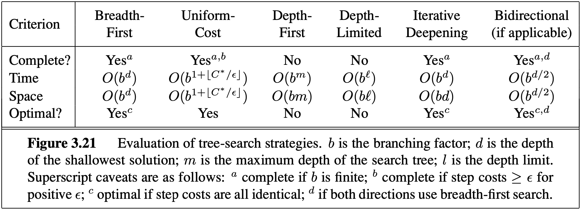
• Search algorithms’ performance are evaluated in four ways:
  • Completeness: Is the algorithm guaranteed to find a solution when there is one?
  • Optimality: Does the strategy find the optimal solution?
  • Time complexity: How long does it take to find a solution?
  • Space complexity: How much memory is needed to perform the search?
• Uninformed Search. Strategies have no additional information about states beyond that provided in the problem definition. All they can do is generate successors and distinguish a goal state from a non-goal state. All search strategies are distinguished by the order in which nodes are expanded. Strategies that know whether one non-goal state is “more promising” than another are called informed search or heuristic search strategies.
  • Breadth-first search is a simple strategy in which the root node is expanded first, then all the successors of the root node are expanded next, then their successors, and so on. This is achieved very simply by using a FIFO queue for the frontier. The goal test is applied to each node when it is generated rather than when it is selected for expansion. BFS is optimal if the path cost is a nondecreasing function of the depth of the node. The most common such scenario is that all actions have the same cost. Imagine searching a uniform tree where every state has $b$ successors. Also, suppose that the solution is at depth $d$. Time and space complexities are $O(b^d)$. Lessons to be learnt from BFS: First, the memory requirements are a bigger problem for breadth-first search than is the execution time. Second lesson is that time is still a major factor.
  • Uniform-cost search expands the node n with the lowest path cost $g(n)$. This is done by storing the frontier as a priority queue ordered by $g$. In addition to the ordering of the queue by path cost, there are two other significant differences from breadth-first search. The first is that the goal test is applied to a node when it is selected for expansion rather than when it is first generated. The reason is that the first goal node that is generated may be on a suboptimal path. The second difference is that a test is added in case a better path is found to a node currently on the frontier. UCS is optimal in general. Uniform-cost search does not care about the number of steps a path has, but only about their total cost. Therefore, it will get stuck in an infinite loop if there is a path with an infinite sequence of zero-cost actions—for example, a sequence of NoOp actions.
  • Depth-first search always expands the deepest node in the current frontier of the search tree. Whereas breadth-first-search uses a FIFO queue, depth-first search uses a LIFO queue. DFS is not optimal. A depth-first tree search, on the other hand, may generate all of the $O(b^m)$ nodes in the search tree, where $m$ is the maximum depth of any node; this can be much greater than the size of the state space. Note that $m$ itself can be much larger than $d$ (the depth of the shallowest solution) and is infinite if the tree is unbounded. For a state space with branching factor $b$ and maximum depth $m$, depth-first search requires storage of only $O(bm)$ nodes, which is DFS’s advantage over BFS. A variant of depth-first search called backtracking search uses still less memory. In backtracking, only one successor is generated at a time rather than all successors; each partially expanded node remembers which successor to generate next. In this way, only $O(m)$ memory is needed rather than $O(bm)$.
  • Depth-limited search nodes at depth $l$ are treated as if they have no successors, which solves the infinite-path problem. Its time complexity is $O(b^l)$ and its space complexity is $O(bl)$. Depth-first search can be viewed as a special case of depth-limited search with $l = \infty$.
  • Iterative deepening DFS combines the benefits of depth-first and breadth-first search. Like depth-first search, its memory requirements are modest: $O(bd)$ to be precise. Like breadth-first search, it is complete when the branching factor is finite and optimal when the path cost is a nondecreasing function of the depth of the node. Iterative deepening search may seem wasteful because states are generated multiple times. It turns out this is not too costly. The reason is that in a search tree with the same (or nearly the same) branching factor at each level, most of the nodes are in the bottom level, so it does not matter much that the upper levels are generated multiple times, which gives a time complexity of $O(b^d)$.
  • Bidirectional search to run two simultaneous searches—one forward from the initial state and the other backward from the goal—hoping that the two searches meet in the middle. The motivation is that $b^{d/2} + b^{d/2}$ is much less than $b^d$. Bidirectional search is implemented by replacing the goal test with a check to see whether the frontiers of the two searches intersect; if they do, a solution has been found. The time complexity of bidirectional search using breadth-first searches in both directions is $O(b^{d/2})$. The space complexity is also $O(b^{d/2})$. We can reduce this by roughly half if one of the two searches is done by iterative deepening, but at least one of the frontiers must be kept in memory so that the intersection check can be done. This space requirement is the most significant weakness of bidirectional search.
  • Comparing uninformed search strategies
• Informed Search Strategies. Most best-first algorithms include as a component of f a heuristic function, denoted $h(n)$: $h(n) = \text{estimated cost of the cheapest path from the state at node n to a goal state.}$ (Notice that $h(n)$ takes a node as input, but, unlike $g(n)$, it depends only on the state at that node.) If $n$ is a goal node, then $h(n) = 0$.

  • Greedy best-first search tries to expand the node that is closest to the goal, on the grounds that this is likely to lead to a solution quickly. Thus, it evaluates nodes by using just the heuristic function; that is, $f (n) = h(n)$. Greedy best-first tree search is also incomplete even in a finite state space, much like depth-first search. The worst-case time and space complexity for the tree version is $O(b^m)$, where $m$ is the maximum depth of the search space.

  • $A$ search: Minimizing the total estimated solution cost.* It evaluates nodes by combining $g(n)$, the cost to reach the node, and $h(n)$, the cost to get from the node to the goal: $$f(n) = g(n) + h(n)$$ Since $g(n)$ gives the path cost from the start node to node $n$, and $h(n)$ is the estimated cost of the cheapest path from n to the goal, we have $$f (n) = \text{estimated cost of the cheapest solution through $n$}$$ Thus, if we are trying to find the cheapest solution, a reasonable thing to try first is the node with the lowest value of $g(n) + h(n)$. $A*$ search is both complete and optimal.

  • Conditions for optimality: Admissibility and consistency The first condition we require for optimality is that $h(n)$ be an admissible heuristic. An admissible heuristic is one that never overestimates the cost to reach the goal. Because $g(n)$ is the actual cost to reach n along the current path, and $f (n) = g(n) + h(n)$, we have as an immediate consequence that $f(n)$ never overestimates the true cost of a solution along the current path through $n$. Admissible heuristics are by nature optimistic because they think the cost of solving the problem is less than it actually is. A second, slightly stronger condition called consistency (or sometimes monotonicity) is required only for applications of $A*$ to graph search. A heuristic $h(n)$ is consistent if, for every node $n$ and every successor $n’$ of $n$ generated by any action $a$, the estimated cost of reaching the goal from $n$ is no greater than the step cost of getting to $n’$ plus the estimated cost of reaching the goal from $n’$: $$ h(n) \leq c(n, a, n’) + h(n’) $$ For an admissible heuristic, the inequality makes perfect sense: if there were a route from $n$ to $G$ via $n’$ that was cheaper than $h(n)$, that would violate the property that $h(n)$ is a lower bound on the cost to reach $G$.

  • Optimality of A* the tree-search version of $A*$ is optimal if $h(n)$ is admissible, while the graph-search version is optimal if $h(n)$ is consistent. It follows that the sequence of nodes expanded by $A*$ using GRAPH-SEARCH is in nondecreasing order of $f(n)$. Hence, the first goal node selected for expansion must be an optimal solution because $f$ is the true cost for goal nodes (which have $h = 0$) and all later goal nodes will be at least as expensive. If $C*$ is the cost of the optimal solution path, then we can say the following:

    • $A*$ expands all nodes with $f(n) < C*$
    • $A*$ might then expand some of the nodes right on the “goal contour” (where $f(n) = C*$) before selecting a goal node.
    • $A*$ expands no nodes with $f(n) > C*$

    No other optimal algorithm is guaranteed to expand fewer nodes than $A*$. The catch is that, for most problems, the number of states within the goal contour search space is still exponential in the length of the solution. The complexity of $A*$ often makes it impractical to insist on finding an optimal solution. One can use variants of $A*$ that find suboptimal solutions quickly, or one can sometimes design heuristics that are more accurate but not strictly admissible. In any case, the use of a good heuristic still provides enormous savings compared to the use of an uninformed search.

  • Memory-bounded heuristic search. The simplest way to reduce memory requirements for $A*$ is to adapt the idea of iterative deepening to the heuristic search context, resulting in the iterative-deepening $A*$ (IDA*). Recursive best-first search (RBFS) is a simple recursive algorithm that attempts to mimic the operation of standard best-first search, but using only linear space. RBFS is somewhat more efficient than IDA*, but still suffers from excessive node regeneration. Like $A*$ tree search, RBFS is an optimal algorithm if the heuristic function h(n) is admissible. Its space complexity is linear in the depth of the deepest optimal solution, but its time complexity is rather difficult to characterize: it depends both on the accuracy of the heuristic function and on how often the best path changes as nodes are expanded. IDA* and RBFS suffer from using too little memory. SMA* proceeds just like $A*$, expanding the best leaf until memory is full. At this point, it cannot add a new node to the search tree without dropping an old one. SMA* always drops the worst leaf node—the one with the highest f-value. Like RBFS, SMA* then backs up the value of the forgotten node to its parent. In this way, the ancestor of a forgotten subtree knows the quality of the best path in that subtree. With this information, SMA* regenerates the subtree only when all other paths have been shown to look worse than the path it has forgotten. SMA* is complete if there is any reachable solution—that is, if d, the depth of the shallowest goal node, is less than the memory size (expressed in nodes). It is optimal if any optimal solution is reachable; otherwise, it returns the best reachable solution.

4. Beyond Classical Search

• Section 3 addressed a single category of problems: observable, deterministic, known environments where the solution is a sequence of actions. In this section, when these assumptions are relaxed are covered.
• Local search two key advantages: (1) they use very little memory—usually a constant amount; and (2) they can often find reasonable solutions in large or infinite (continuous) state spaces for which systematic algorithms are unsuitable.
• Local search algorithms are useful for solving pure optimization problems, in which the aim is to find the best state according to an objective function.
• State-space landscape. A landscape has both “location” (defined by the state) and “elevation” (defined by the value of the heuristic cost function or objective function). If elevation corresponds to cost, then the aim is to find the lowest valley—a global minimum; if elevation corresponds to an objective function, then the aim is to find the highest peak—a global maximum.
• A complete local search algorithm always finds a goal if one exists; an optimal algorithm always finds a global minimum/maximum.
• Hill-climbing search. It is simply a loop that continually moves in the direction of increasing value—that is, uphill. It terminates when it reaches a “peak” where no neighbor has a higher value. Hill climbing does not look ahead beyond the immediate neighbors of the current state. Hill climbing is sometimes called greedy local search because it grabs a good neighbor state without thinking ahead about where to go next. It often gets stuck for the following reasons:
  • Local maxima.
  • Ridges.
  • Plateaux.
• Stochastic hill climbing chooses at random from among the uphill moves; the probability of selection can vary with the steepness of the uphill move. This usually converges more slowly than steepest ascent, but in some state landscapes, it finds better solutions.
• First-choice hill climbing implements stochastic hill climbing by generating successors randomly until one is generated that is better than the current state. This is a good strategy when a state has many (e.g., thousands) of successors.
• Random-restart hill climbing conducts a series of hill-climbing searches from randomly generated initial states, until a goal is found. It is trivially complete with probability approaching 1, because it will eventually generate a goal state as the initial state. If each hill-climbing search has a probability $p$ of success, then the expected number of restarts required is $1/p$.
• Simulated annealing solution is to start by shaking hard (i.e., at a high temperature) and then gradually reduce the intensity of the shaking (i.e., lower the temperature). The innermost loop of the simulated-annealing algorithm is quite similar to hill climbing. Instead of picking the best move, however, it picks a random move. If the move improves the situation, it is always accepted. Otherwise, the algorithm accepts the move with some probability less than 1. The probability decreases exponentially with the “badness” of the move—the amount $\Delta E$ by which the evaluation is worsened. The probability also decreases as the “temperature” $T$ goes down: “bad” moves are more likely to be allowed at the start when $T$ is high, and they become more unlikely as $T$ decreases. If the schedule lowers $T$ slowly enough, the algorithm will find a global optimum with probability approaching 1.
• Local beam search keeps track of $k$ states rather than just one. It begins with $k$ randomly generated states. At each step, all the successors of all $k$ states are generated. If any one is a goal, the algorithm halts. Otherwise, it selects the $k$ best successors from the complete list and repeats. In a local beam search, useful information is passed among the parallel search threads.
• Genetic algorithm (or GA) is a variant of stochastic beam search in which successor states are generated by combining two parent states rather than by modifying a single state. GAs begin with a set of $k$ randomly generated states, called the population. Each state is rated by the objective function, or (in GA terminology) the fitness function. A fitness function should return higher values for better states. Then two pairs are selected at random for reproduction, in accordance with the probability in previous step. For each pair to be mated, a crossover point is chosen randomly from the positions in the string. Then offspring themselves are created by crossing over the parent strings at the crossover point. It is often the case that the population is quite diverse early on in the process, so crossover (like simulated annealing) frequently takes large steps in the state space early in the search process and smaller steps later on when most individuals are quite similar. Finally each location is subject to random mutation with a small independent probability.
• An optimization problem is constrained if solutions must satisfy some hard constraints on the values of the variables.
• Searching with Nondeterministic Actions. Solutions for nondeterministic problems can contain nested if–then–else statements; this means that they are trees rather than sequences. In a deterministic environment, the only branching is introduced by the agent’s own choices in each state. We call these nodes OR nodes. In a nondeterministic environment, branching is also introduced by the environment’s choice of outcome for each action. We call these nodes AND nodes. A solution for an AND–OR search problem is a subtree that (1) has a goal node at every leaf, (2) specifies one action at each of its OR nodes, and (3) includes every outcome branch at each of its AND nodes.
• Searching with Partial Observations. To solve sensorless problems, we search in the space of belief states rather than physical states. Suppose the underlying physical problem $P$ is defined by $ACTIONS_P$ , $RESULT_P$ , $GOAL-TEST_P$ , and $STEP-COST_P$ . Then we can define the corresponding sensorless problem as follows:
  • Belief states: The entire belief-state space contains every possible set of physical states. If $P$ has $N$ states, then the sensorless problem has up to $2^N$ states, although many may be unreachable from the initial state.
  • Initial state: Typically the set of all states in $P$ , although in some cases the agent will have more knowledge than this.
  • Actions: This is slightly tricky. Suppose the agent is in belief state $b = {s1, s2}$, but $ACTIONS_P (s_1) \neq ACTIONS_P (s_2)$; then the agent is unsure of which actions are legal. It can either take and union of the actions or the intersection.
  • Transition model: The agent doesn’t know which state in the belief state is the right one; so as far as it knows, it might get to any of the states resulting from applying the action to one of the physical states in the belief state.
  • Goal test: The agent wants a plan that is sure to work, which means that a belief state satisfies the goal only if all the physical states in it satisfy $GOAL-TEST_P$.
  • Path cost: This is also tricky. If the same action can have different costs in different states, then the cost of taking an action in a given belief state could be one of several values. The preceding definitions enable the automatic construction of the belief-state problem formulation from the definition of the underlying physical problem. Once this is done, we can apply any of the search algorithms.
• Online search. Online search is a good idea in dynamic or semidynamic domains—domains where there is a penalty for sitting around and computing too long. Online search is a necessary idea for unknown environments, where the agent does not know what states exist or what its actions do. In this state of ignorance, the agent faces an exploration problem and must use its actions as experiments in order to learn enough to make deliberation worthwhile. We stipulate that the agent knows only the following:
  • $ACTIONS(s)$, which returns a list of actions allowed in state s
  • The step-cost function $c(s, a, s’)$—note that this cannot be used until the agent knows that $s’$ is the outcome
  • $GOAL-TEST(s)$ Note in particular that the agent cannot determine $RESULT(s, a)$ except by actually being in $s$ and doing $a$. Typically, the agent’s objective is to reach a goal state while minimizing cost. The cost is the total path cost of the path that the agent actually travels. It is common to compare this cost with the path cost of the path the agent would follow if it knew the search space in advance—that is, the actual shortest path. In the language of online algorithms, this is called the competitive ratio; we would like it to be as small as possible. No algorithm can avoid dead ends in all state spaces. No bounded competitive ratio can be guaranteed if there are paths of unbounded cost.

5. Adversarial Search

• A game can be formally defined as a kind of search problem with the following elements:
  • $S_0$: The initial state, which specifies how the game is set up at the start.
  • $PLAYER(s)$: Defines which player has the move in a state.
  • $ACTIONS(s)$: Returns the set of legal moves in a state.
  • $RESULT(s, a)$: The transition model, which defines the result of a move.
  • $TERMINAL-TEST(s)$: A terminal test, which is true when the game is over and false otherwise. States where the game has ended are called terminal states.
  • $UTILITY(s, p)$: A utility function (also called an objective function or payoff function), defines the final numeric value for a game that ends in terminal state $s$ for a player $p$. In chess, the outcome is a win, loss, or draw, with values $+1$, $0$, or $1/2$ . Some games have a wider variety of possible outcomes. A zero-sum game is (confusingly) defined as one where the total payoff to all players is the same for every instance of the game. Chess is zero-sum because every game has payoff of either $0 + 1$, $1 + 0$ or $1/2 + 1/2$. “Constant-sum” would have been a better term, but zero-sum is traditional and makes sense if you imagine each player is charged an entry fee of $1/2$.
• Given a choice, MAX prefers to move to a state of maximum value, whereas MIN prefers a state of minimum value. The minimax algorithm performs a complete depth-first exploration of the game tree. If the maximum depth of the tree is $m$ and there are $b$ legal moves at each point, then the time complexity of the minimax algorithm is $O(b^m)$. The space complexity is $O(bm)$ for an algorithm that generates all actions at once, or $O(m)$ for an algorithm that generates actions one at a time.
• Alpha-Beta Pruning. The problem with minimax search is that the number of game states it has to examine is exponential in the depth of the tree. When applied to a standard minimax tree, it returns the same move as minimax would, but prunes away branches that cannot possibly influence the final decision. Minimax search is depth-first, so at any one time we just have to consider the nodes along a single path in the tree. Alpha–beta pruning gets its name from the following two parameters that describe bounds on the backed-up values that appear anywhere along the path:
  • $\alpha$ = the value of the best (i.e., highest-value) choice we have found so far at any choice point along the path for MAX.
  • $\beta$ = the value of the best (i.e., lowest-value) choice we have found so far at any choice point along the path for MIN. The effectiveness of alpha–beta pruning is highly dependent on the order in which the states are examined. This suggests that it might be worthwhile to try to examine first the successors that are likely to be best. If this can be done, then it turns out that alpha–beta needs to examine only $O(b ^{m/2})$ nodes to pick the best move, instead of $O(b^m)$ for minimax. Alpha–beta can solve a tree roughly twice as deep as minimax in the same amount of time. If successors are examined in random order rather than best-first, the total number of nodes examined will be roughly $O(b^{3m/4})$ for moderate $b$.
• Evaluation functions should order the terminal states in the same way as the true utility function: states that are wins must evaluate better than draws, which in turn must be better than losses. Otherwise, an agent using the evaluation function might err even if it can see ahead all the way to the end of the game. Second, the computation must not take too long! (The whole point is to search faster.) Third, for nonterminal states, the evaluation function should be strongly correlated with the actual chances of winning. Most evaluation functions work by calculating various features of the state. The features, taken together, define various categories or equivalence classes of states: the states in each category have the same values for all the features. The evaluation function should be applied only to positions that are quiescent—that is, unlikely to exhibit wild swings in value in the near future.
• Stochastic games. Positions do not have definite minimax values. Instead, we can only calculate the expected value of a position: the average over all possible outcomes of the chance nodes. As with minimax, the obvious approximation to make with expectiminimax is to cut the search off at some point and apply an evaluation function to each leaf. One might think that evaluation functions for games such as backgammon should be just like evaluation functions for chess—they just need to give higher scores to better positions. But in fact, the presence of chance nodes means that one has to be more careful about what the evaluation values mean. If the program knew in advance all the dice rolls that would occur for the rest of the game, solving a game with dice would be just like solving a game without dice, which minimax does in $O(b^m)$ time, where $b$ is the branching factor and $m$ is the maximum depth of the game tree. Because expectiminimax is also considering all the possible dice-roll sequences, it will take $O(b^m n^m)$, where $n$ is the number of distinct rolls.
• Partially observable games. Given a current belief state, one may ask, “Can I win the game?” For a partially observable game, the notion of a strategy is altered; instead of specifying a move to make for each possible move the opponent might make, we need a move for every possible percept sequence that might be received. In addition to guaranteed checkmates, Kriegspiel admits an entirely new concept that makes no sense in fully observable games: probabilistic checkmate. Such checkmates are still required to work in every board state in the belief state; they are probabilistic with respect to randomization of the winning player’s moves.

6. Constraint Satisfaction Problems

• A constraint satisfaction problem consists of three components, $X$, $D$, and $C$:
  • $X$ is a set of variables, ${X_1,…,X_n}$.
  • $D$ is a set of domains, ${D_1, . . . , D_n}$, one for each variable.
  • $C$ is a set of constraints that specify allowable combinations of values. Each domain $D_i$ consists of a set of allowable values, ${v_1,…,v_k}$ for variable $X_i$. Each constraint $C_i$ consists of a pair $<scope , rel>$, where $scope$ is a tuple of variables that participate in the constraint and $rel$ is a relation that defines the values that those variables can take on. A relation can be represented as an explicit list of all tuples of values that satisfy the constraint, or as an abstract relation that supports two operations: testing if a tuple is a member of the relation and enumerating the members of the relation.
• To solve a CSP, we need to define a state space and the notion of a solution. Each state in a CSP is defined by an assignment of values to some or all of the variables, ${X_i = v_i, X_j = v_j , …}$. An assignment that does not violate any constraints is called a consistent or legal assignment. A complete assignment is one in which every variable is assigned, and a solution to a CSP is a consistent, complete assignment. A partial assignment is one that assigns values to only some of the variables.
• Why formulate a problem as a CSP? One reason is that the CSPs yield a natural representation for a wide variety of problems; if you already have a CSP-solving system, it is often easier to solve a problem using it than to design a custom solution using another search technique. In addition, CSP solvers can be faster than state-space searchers because the CSP solver can quickly eliminate large swatches of the search space. With CSPs, once we find out that a partial assignment is not a solution, we can immediately discard further refinements of the partial assignment. Furthermore, we can see why the assignment is not a solution—we see which variables violate a constraint—so we can focus attention on the variables that matter. As a result, many problems that are intractable for regular state-space search can be solved quickly when formulated as a CSP.
• Constraint hypergraph. constraints can be represented in a constraint hypergraph. A hypergraph consists of ordinary nodes (the circles in the figure) and hypernodes (the squares), which represent n-ary constraints.
• Preference constraints indicates which solutions are preferred, such problems are called constraint optimization problem, or COP.
• Constraint propagation. In regular state-space search, an algorithm can do only one thing: search. In CSPs there is a choice: an algorithm can search (choose a new variable assignment from several possibilities) or do a specific type of inference called constraint propagation: using the constraints to reduce the number of legal values for a variable, which in turn can reduce the legal values for another variable, and so on.
• Node consistency. A single variable (corresponding to a node in the CSP network) is node-consistent if all the values in the variable’s domain satisfy the variable’s unary constraints.
• Arc consistency. A variable in a CSP is arc-consistent if every value in its domain satisfies the variable’s binary constraints. More formally, $X_i$ is arc-consistent with respect to another variable $X_j$ if for every value in the current domain $D_i$ there is some value in the domain $D_j$ that satisfies the binary constraint on the arc $(X_i, X_j)$.
• Path consistency. A two-variable set ${X_i,X_j}$ is path-consistent with respect to a third variable $X_m$ if, for every assignment ${X_i = a, X_j = b}$ consistent with the constraints on ${X_i , X_j}$, there is an assignment to $X_m$ that satisfies the constraints on ${X_i, X_m}$ and ${X_m, X_j}$. This is called path consistency because one can think of it as looking at a path from $X_i$ to $X_j$ with $X_m$ in the middle.
• $K$-consistency. A CSP is $k$-consistent if, for any set of $k - 1$ variables and for any consistent assignment to those variables, a consistent value can always be assigned to any $k$th variable. 1-consistency says that, given the empty set, we can make any set of one variable consistent: this is what we called node consistency. 2-consistency is the same as arc consistency. For binary constraint networks, 3-consistency is the same as path consistency.
• Commutativity. A problem is commutative if the order of application of any given set of actions has no effect on the outcome. CSPs are commutative because when assigning values to variables, we reach the same partial assignment regardless of order. Therefore, we need only consider a single variable at each node in the search tree.
• Backtracking search. The term backtracking search is used for a depth-first search that chooses values for one variable at a time and backtracks when a variable has no legal values left to assign. It repeatedly chooses an unassigned variable, and then tries all values in the domain of that variable in turn, trying to find a solution. If an inconsistency is detected, then BACKTRACK returns failure, causing the previous call to try another value.
• Variable and value ordering. Intuitive idea—choosing the variable with the fewest “legal” values—is called the minimum-remaining-values (MRV) heuristic. The MRV heuristic doesn’t help at all in choosing the first region to color in Australia, because initially every region has three legal colors. In this case, the degree heuristic comes in handy. It attempts to reduce the branching factor on future choices by selecting the variable that is involved in the largest number of constraints on other unassigned variables. Once a variable has been selected, the algorithm must decide on the order in which to examine its values. For this, the least-constraining-value heuristic can be effective in some cases. It prefers the value that rules out the fewest choices for the neighboring variables in the constraint graph.
• Local search for CSPs. Local search algorithms turn out to be effective in solving many CSPs. They use a complete-state formulation: the initial state assigns a value to every variable, and the search changes the value of one variable at a time. In choosing a new value for a variable, the most obvious heuristic is to select the value that results in the minimum number of conflicts with other variables—the min-conflicts heuristic. Roughly speaking, n-queens is easy for local search because solutions are densely distributed throughout the state space.

7. Logical Agents

• Knowledge base. A knowledge base is a set of sentences. Each sentence is expressed in a language called a knowledge representation language and represents some assertion about the world. Sometimes we dignify a sentence with the name axiom, when the sentence is taken as given without being derived from other sentences. There must be a way to add new sentences to the knowledge base and a way to query what is known. The standard names for these operations are TELL and ASK, respectively. Both operations may involve inference—that is, deriving new sentences from old. Inference must obey the requirement that when one ASKs a question of the knowledge base, the answer should follow from what has been told (or TELLed) to the knowledge base previously. The agent maintains a knowledge base, KB, which may initially contain some background knowledge. Each time the agent program is called, it does three things. First, it TELLs the knowledge base what it perceives. Second, it ASKs the knowledge base what action it should perform. In the process of answering this query, extensive reasoning may be done about the current state of the world, about the outcomes of possible action sequences, and so on. Third, the agent program TELLs the knowledge base which action was chosen, and the agent executes the action.

• The Wumpus world. It is discrete, static, and single-agent. It is sequential, because rewards may come only after many actions are taken. It is partially observable, because some aspects of the state are not directly perceivable: the agent’s location, the wumpus’s state of health, and the availability of an arrow. As for the locations of the pits and the wumpus: we could treat them as unobserved parts of the state that happen to be immutable—in which case, the transition model for the environment is completely known. The agent’s initial knowledge base contains the rules of the environment. Note that in each case for which the agent draws a conclusion from the available information, that conclusion is guaranteed to be correct if the available information is correct. This is a fundamental property of logical reasoning.

• Logic. Knowledge bases consist of sentences. These sentences are expressed according to the syntax of the representation language, which specifies all the sentences that are well formed. A logic must also define the semantics or meaning of sentences. The semantics defines the truth of each sentence with respect to each possible world. When we need to be precise, we use the term model in place of “possible world.” Whereas possible worlds might be thought of as (potentially) real environments that the agent might or might not be in, models are mathematical abstractions, each of which simply fixes the truth or falsehood of every relevant sentence. If a sentence $\alpha$ is true in model $m$, we say that $m$ satisfies $\alpha$ or sometimes $m$ is a model of $\alpha$. We use the notation $M(\alpha)$ to mean the set of all models of $\alpha$. Formal definition of entailment is this: $\alpha \models \beta$ if and only if, in every model in which $\alpha$ is true, $\beta$ is also true. Using the notation just introduced, we can write: $$\alpha \models \beta ; \text{iff} ; M(\alpha) \subseteq M(\beta)$$ Model checking enumerates all possible models to check that $\alpha$ is true in all models in which KB is true, that is, that $M(KB) \subseteq M(\alpha)$. If an inference algorithm $i$ can derive $\alpha$ from KB, we write: $$KB \vdash_i \alpha$$ which is pronounced “$\alpha$ is derived from KB by $i$” or “$i$ derives $\alpha$ from KB”. An inference algorithm that derives only entailed sentences is called sound or truth-preserving. The property of completeness is also desirable: an inference algorithm is complete if it can derive any sentence that is entailed. If KB is true in the real world, then any sentence $\alpha$ derived from KB by a sound inference procedure is also true in the real world. The final issue to consider is grounding—the connection between logical reasoning processes and the real environment in which the agent exists. In particular, how do we know that KB is true in the real world? (After all, KB is just “syntax” inside the agent’s head.)

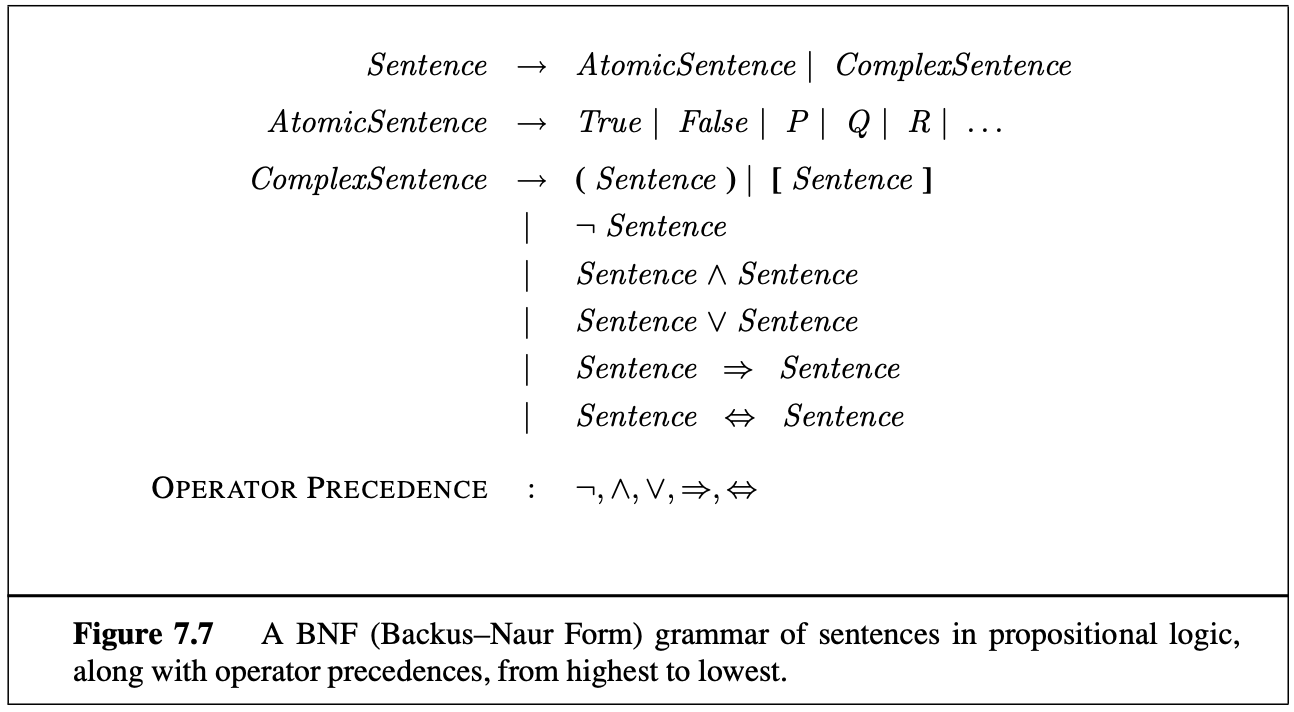
• Propositional Logic: A Very Simple Logic. The syntax of propositional logic defines the allowable sentences. The atomic sentences consist of a single proposition symbol. Complex sentences are constructed from simpler sentences, using parentheses and logical connectives. There are five connectives in common use:

  • $\neg$ (not). A sentence such as $\neg W_1$ is called the negation of $W_1$. A literal is either an atomic sentence (a positive literal) or a negated atomic sentence (a negative literal).
  • $\wedge$ (and). A sentence whose main connective is $\wedge$, such as $W_1 \wedge P_1$, is called a conjunction.
  • $\vee$ (or). A sentence using $\vee$, such as $(W_1 \wedge P_1) \vee W_2$, is a disjunction of the disjuncts.
  • $\implies$ (implies). A sentence such as $(W_1 \wedge P_1) \implies W_2$ is called an implication (or conditional). Its premise or antecedent is $(W_1 \wedge P_1)$, and its conclusion or consequent is $W_2$. Implications are also known as rules or if–then statements.
  • $\iff$ (if and only if). The sentence $W_1 \iff W_2$ is a biconditional.

  

  The semantics for propositional logic must specify how to compute the truth value of any sentence, given a model. We need to specify how to compute the truth of atomic sentences and how to compute the truth of sentences formed with each of the five connectives. Atomic sentences are easy:

  • True is true in every model and False is false in every model.

  For complex sentences, we have five rules:

  • $\neg P$ is true iff $P$ is false in $m$.
  • $P \wedge Q$ is true iff both $P$ and $Q$ are true in $m$.
  • $P \vee Q$ is true iff either $P$ or $Q$ is true in $m$.
  • $P \implies Q$ is true unless $P$ is true and $Q$ is false in $m$.
  • $P \iff Q$ is true iff $P$ and $Q$ are both true or both false in $m$.

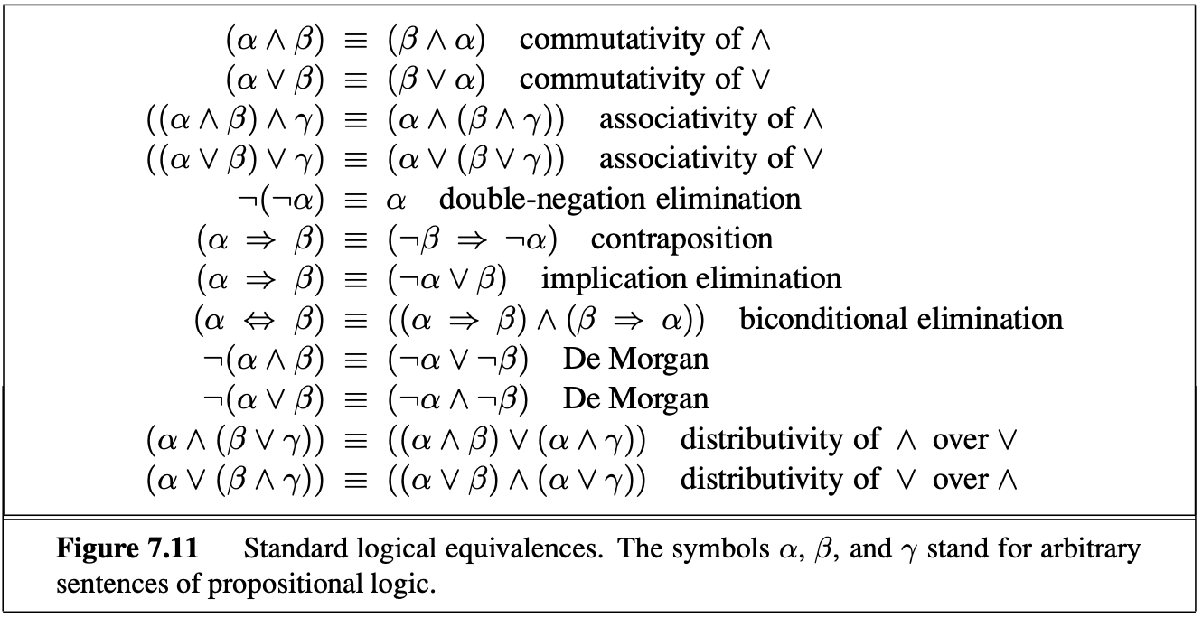
• Propositional Theorem Proving. Logical equivalence: two sentences $\alpha$ and $\beta$ are logically equivalent if they are true in the same set of models. We write this as $\alpha \equiv \beta$. We can also say two sentences are logically equivalent if each of them entails the other. A sentence is valid if it is true in all models. A sentence is satisfiable if it is true in, or satisfied by, some model.

• Inference and proofs. The best-known rule is called Modus Ponens: whenever any sentences of the form $\alpha \implies \beta$ and $\alpha$ are given, then the sentence $\beta$ can be inferred. And-Elimination: from $\alpha \wedge \beta$, $\alpha$ can be inferred. One final property of logical systems is monotonicity, which says that the set of entailed sentences can only increase as information is added to the knowledge base.

8. First-Order Logic

• Compositionality. In a compositional language, the meaning of a sentence is a function of the meaning of its parts. For example, the meaning of $S_1 \wedge S_2$ is related to the meanings of $S_1$ and $S_2$.
• From the viewpoint of formal logic, representing the same knowledge in two different ways makes absolutely no difference; the same facts will be derivable from either representation. In practice, however, one representation might require fewer steps to derive a conclusion, meaning that a reasoner with limited resources could get to the conclusion using one representation but not the other.
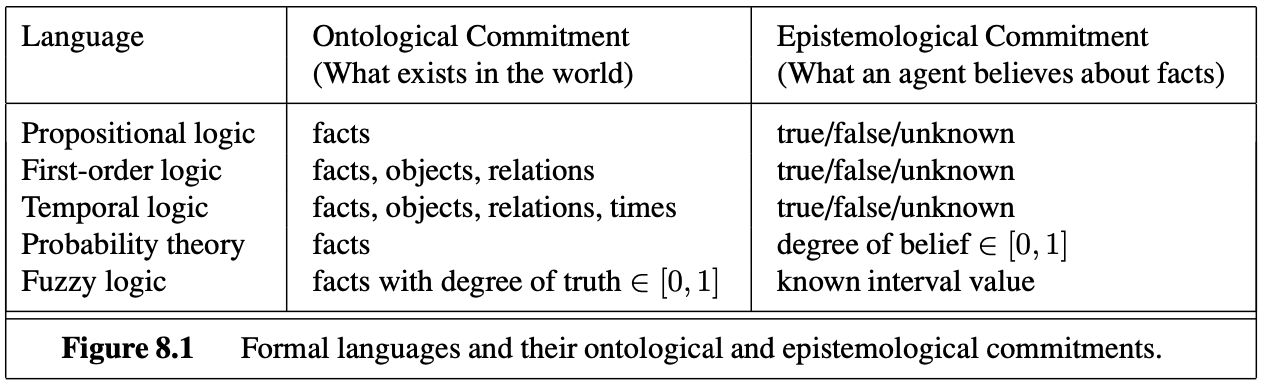
• The primary difference between propositional and first-order logic lies in the ontological commitment made by each language—that is, what it assumes about the nature of reality. Mathematically, this commitment is expressed through the nature of the formal models with respect to which the truth of sentences is defined. For example, propositional logic assumes that there are facts that either hold or do not hold in the world. Each fact can be in one of two states: true or false, and each model assigns true or false to each proposition symbol. First-order logic assumes more; namely, that the world consists of objects with certain relations among them that do or do not hold. The formal models are correspondingly more complicated than those for propositional logic.
• Models for first-order logic are much more interesting. First, they have objects in them! The domain of a model is the set of objects or domain elements it contains. The domain is required to be nonempty—every possible world must contain at least one object. Mathematically speaking, it doesn’t matter what these objects are—all that matters is how many there are in each particular model.
• Symbols and interpretations. The basic syntactic elements of first-order logic are the symbols that stand for objects, relations, and functions. The symbols, therefore, come in three kinds: constant symbols, which stand for objects; predicate symbols, which stand for relations; and function symbols, which stand for functions. In addition to its objects, relations, and functions, each model includes an interpretation that specifies exactly which objects, relations and functions are referred to by the constant, predicate, and function symbols.
• Terms are logical expressions that refer to objects. Constant symbols are therefore terms, but it is not always convenient to have a distinct symbol to name every object.
• Atomic sentences are formed from a predicate symbol optionally followed by a parenthesized list of terms. An atomic sentence is true in a given model if the relation referred to by the predicate symbol holds among the objects referred to by the arguments.
• Quantifiers. First-order logic contains two standard quantifiers, called universal, $\forall$ and existential, $\exists$. Connections between the two are as follows: $$\forall x \neg Likes(x, soup) \text{ is equivalent to } \neg \exists Likes(x, soup)$$

9. Inference in First-Order Logic

• Modus ponens is a rule of inference. It can be summarized as “$P$ implies $Q$ and $P$ is asserted to be true, therefore $Q$ must be true”.
• A lifted version of Modus Ponens uses unification to provide a natural and powerful inference rule, generalized Modus Ponens. The forward-chaining and backward-chaining algorithms apply this rule to sets of definite clauses. Generalized Modus Ponens is complete for definite clauses, although the entailment problem is semidecidable. For Datalog knowledge bases consisting of function-free definite clauses, entailment is decidable. Forward chaining is used in deductive databases, where it can be combined with relational database operations. It is also used in production systems, which perform efficient updates with very large rule sets. Forward chaining is complete for Datalog and runs in polynomial time. Backward chaining is used in logic programming systems, which employ sophisticated compiler technology to provide very fast inference. Backward chaining suffers from redundant inferences and infinite loops; these can be alleviated by memoization. Prolog, unlike first-order logic, uses a closed world with the unique names assumption and negation as failure. These make Prolog a more practical programming language, but bring it further from pure logic. The generalized resolution inference rule provides a complete proof system for first-order logic, using knowledge bases in conjunctive normal form. Several strategies exist for reducing the search space of a resolution system without compromising completeness. One of the most important issues is dealing with equality; we showed how demodulation and paramodulation can be used. Efficient resolution-based theorem provers have been used to prove interesting mathematical theorems and to verify and synthesize software and hardware.

10. Classical Planning

• Planning is devising a plan of action to achieve one’s goals and is a critical part of AI.
• We say that action $a$ is applicable in state $s$ if the preconditions are satisfied by $s$. The result of executing action $a$ in state $s$ is defined as a state $s’$ which is represented by the set of fluents formed by starting with $s$. A specific problem within the domain is defined with the addition of an initial state and a goal. The initial state is a conjunction of ground atoms. The goal is just like a precondition: a conjunction of literals (positive or negative) that may contain variables. Now we have defined planning as a search problem: we have an initial state, an ACTIONS function, a RESULT function, and a goal test.
• PlanSAT is the question of whether there exists any plan that solves a planning problem. Bounded PlanSAT asks whether there is a solution of length $k$ or less; this can be used to find an optimal plan. The first result is that both decision problems are decidable for classical planning.
• Now that we have shown how a planning problem maps into a search problem, we can solve planning problems with any of the heuristic search algorithms from Chapter 3 or a local search algorithm from Chapter 4 (provided we keep track of the actions used to reach the goal).
• Why forward-search assumed to be inefficient? First, forward search is prone to exploring irrelevant actions. Second, planning problems often have large state spaces.
• Neither forward nor backward search is efficient without a good heuristic function. An admissible heuristic can be derived by defining a relaxed problem that is easier to solve. The exact cost of a solution to this easier problem then becomes the heuristic for the original problem.
• Think of a search problem as a graph where the nodes are states and the edges are actions. The problem is to find a path connecting the initial state to a goal state. There are two ways we can relax this problem to make it easier: by adding more edges to the graph, making it strictly easier to find a path, or by grouping multiple nodes together (state abstraction), forming an abstraction of the state space that has fewer states, and thus is easier to search.
• A key idea in defining heuristics is decomposition: dividing a problem into parts, solving each part independently, and then combining the parts. The subgoal independence assumption is that the cost of solving a conjunction of subgoals is approximated by the sum of the costs of solving each subgoal independently.
• Planning graphs. A planning problem asks if we can reach a goal state from the initial state. Suppose we are given a tree of all possible actions from the initial state to successor states, and their successors, and so on. If we indexed this tree appropriately, we could answer the planning question “can we reach state $G$ from state $S_0$” immediately, just by looking it up. The planning graph can’t answer definitively whether $G$ is reachable from $S_0$, but it can estimate how many steps it takes to reach $G$. The estimate is always correct when it reports the goal is not reachable, and it never overestimates the number of steps, so it is an admissible heuristic. A planning graph is polynomial in the size of the planning problem.
• A planning graph, once constructed, is a rich source of information about the problem. First, if any goal literal fails to appear in the final level of the graph, then the problem is unsolvable. Second, we can estimate the cost of achieving any goal literal $g_i$ from state $s$ as the level at which $g_i$ first appears in the planning graph constructed from initial state $s$. It’s called the level cost of $g_i$.
• GraphPlan. The name graphplan is due to the use of a novel planning graph, to reduce the amount of search needed to find the solution from straightforward exploration of the state space graph. In the state space graph:
  • the nodes are possible states,
  • and the edges indicate reachability through a certain action. On the contrary, in Graphplan’s planning graph:
  • the nodes are actions and atomic facts, arranged into alternate levels,
  • and the edges are of two kinds:
    • from an atomic fact to the actions for which it is a condition,
    • from an action to the atomic facts it makes true or false. the first level contains true atomic facts identifying the initial state. Lists of incompatible facts that cannot be true at the same time and incompatible actions that cannot be executed together are also maintained. The algorithm then iteratively extends the planning graph, proving that there are no solutions of length $l-1$ before looking for plans of length $l$ by backward chaining: supposing the goals are true, Graphplan looks for the actions and previous states from which the goals can be reached, pruning as many of them as possible thanks to incompatibility information.
• Analysis of planning approaches. Planning combines the two major areas of AI we have covered so far: search and logic. A planner can be seen either as a program that searches for a solution or as one that (constructively) proves the existence of a solution. Sometimes it is possible to solve a problem efficiently by recognizing that negative interactions can be ruled out. We say that a problem has serializable subgoals if there exists an order of subgoals such that the planner can achieve them in that order without having to undo any of the previously achieved subgoals.

11. Planning and Acting in the Real World

• The classical planning representation talks about what to do, and in what order, but the representation cannot talk about time: how long an action takes and when it occurs. We divide the overall problem into a planning phase in which actions are selected, with some ordering constraints, to meet the goals of the problem, and a later scheduling phase, in which temporal information is added to the plan to ensure that it meets resource and deadline constraints.
• Solving scheduling problems. The critical path is that path whose total duration is longest; the path is “critical” because it determines the duration of the entire plan—shortening other paths doesn’t shorten the plan as a whole, but delaying the start of any action on the critical path slows down the whole plan. Actions that are off the critical path have a window of time in which they can be executed.Mathematically speaking, critical-path problems are easy to solve because they are defined as a conjunction of linear inequalities on the start and end times. When we introduce resource constraints, the resulting constraints on start and end times become more complicated. Up to this point, we have assumed that the set of actions and ordering constraints is fixed. Under these assumptions, every scheduling problem can be solved by a nonoverlapping sequence that avoids all resource conflicts, provided that each action is feasible by itself.
• Hierarchical planning. The basic formalism we adopt to understand hierarchical decomposition comes from the area of hierarchical task networks or HTN planning. As in classical planning (Chapter 10), we assume full observability and determinism and the availability of a set of actions, now called primitive actions, with standard precondition–effect schemas. The key additional concept is the high-level action or HLA. Each HLA has one or more possible refinements, into a sequence of actions, each of which may be an HLA or a primitive action (which has no refinements by definition). An HLA refinement that contains only primitive actions is called an implementation of the HLA. An implementation of a high-level plan (a sequence of HLAs) is the concatenation of implementations of each HLA in the sequence. Given the precondition–effect definitions of each primitive action, it is straightforward to determine whether any given implementation of a high-level plan achieves the goal. We can say, then, that a high-level plan achieves the goal from a given state if at least one of its implementations achieves the goal from that state. The “at least one” in this definition is crucial—not all implementations need to achieve the goal, because the agent gets to decide which implementation it will execute. HTN planning is often formulated with a single “top level” action called Act, where the aim is to find an implementation of Act that achieves the goal. The approach leads to a simple algorithm: repeatedly choose an HLA in the current plan and replace it with one of its refinements, until the plan achieves the goal. The hierarchical search algorithm refines HLAs all the way to primitive action sequences to determine if a plan is workable. The notion of reachable sets yields a straightforward algorithm: search among high-level plans, looking for one whose reachable set intersects the goal; once that happens, the algorithm can commit to that abstract plan, knowing that it works, and focus on refining the plan further.
• Planning and acting in nondeterministic domains. Planners deal with factored representations rather than atomic representations. This affects the way we represent the agent’s capability for action and observation and the way we represent belief states—the sets of possible physical states the agent might be in—for unobservable and partially observable environments. To solve a partially observable problem, the agent will have to reason about the percepts it will obtain when it is executing the plan. The percept will be supplied by the agent’s sensors when it is actually acting, but when it is planning it will need a model of its sensors. For a fully observable environment, we would have a Percept axiom with no preconditions for each fluent. A sensorless agent, on the other hand, has no Percept axioms at all. Note that even a sensorless agent can solve the painting problem. A contingent planning agent with sensors can generate a better plan. Finally, an online planning agent might generate a contingent plan with fewer branches at first and deal with problems when they arise by replanning. It could also deal with incorrectness of its action schemas. Whereas a contingent planner simply assumes that the effects of an action always succeed—that painting the chair does the job—a replanning agent would check the result and make an additional plan to fix any unexpected failure, such as an unpainted area or the original color showing through. In classical planning, where the closed-world assumption is made, we would assume that any fluent not mentioned in a state is false, but in sensorless (and partially observable) planning we have to switch to an open-world assumption in which states contain both positive and negative fluents, and if a fluent does not appear, its value is unknown. Thus, the belief state corresponds exactly to the set of possible worlds that satisfy the formula. A heuristic function to guide the search is a piece in sensorless planning puzzle. The meaning of the heuristic function is the same as for classical planning: an estimate (perhaps admissible) of the cost of achieving the goal from the given belief state. With belief states, we have one additional fact: solving any subset of a belief state is necessarily easier than solving the belief state. The decision as to how much of the problem to solve in advance and how much to leave to replanning is one that involves tradeoffs among possible events with different costs and probabilities of occurring. Replanning may also be needed if the agent’s model of the world is incorrect. The model for an action may have a missing precondition—for example, the agent may not know that removing the lid of a paint can often requires a screwdriver; the model may have a missing effect—for example, painting an object may get paint on the floor as well; or the model may have a missing state variable—for example, the model given earlier has no notion of the amount of paint in a can, of how its actions affect this amount, or of the need for the amount to be nonzero. The model may also lack provision for exogenous events such as someone knocking over the paint can.
• Multiagent planning is necessary when there are other agents in the environment with which to cooperate or compete. Joint plans can be constructed, but must be augmented with some form of coordination if two agents are to agree on which joint plan to execute.

12. Knowledge Representation

• Representing abstract concepts is sometimes called ontological engineering. We have elected to use first-order logic to discuss the content and organization of knowledge, although certain aspects of the real world are hard to capture in FOL. The principal difficulty is that most generalizations have exceptions or hold only to a degree. Two major characteristics of general-purpose ontologies distinguish them from collections of special-purpose ontologies:
  • A general-purpose ontology should be applicable in more or less any special-purpose domain (with the addition of domain-specific axioms). This means that no representational issue can be finessed or brushed under the carpet.
  • In any sufficiently demanding domain, different areas of knowledge must be unified, because reasoning and problem solving could involve several areas simultaneously.
• Categories and objects. The organization of objects into categories is a vital part of knowledge representation. There are two choices for representing categories in first-order logic: predicates and objects. Categories serve to organize and simplify the knowledge base through inheritance. If we say that all instances of the category Food are edible, and if we assert that Fruit is a subclass of Food and Apples is a subclass of Fruit, then we can infer that every apple is edible. First-order logic makes it easy to state facts about categories, either by relating objects to categories or by quantifying over their members. Here are some types of facts:
  • An object is a member of a category.
  • A category is a subclass of another category.
  • All members of a category have some properties.
  • Members of a category can be recognized by some properties.
  • A category as a whole has some properties. We say that two or more categories are disjoint if they have no members in common. In both scientific and commonsense theories of the world, objects have height, mass, cost, and so on. The values that we assign for these properties are called measures. The most important aspect of measures is not the particular numerical values, but the fact that measures can be ordered. The real world can be seen as consisting of primitive objects (e.g., atomic particles) and composite objects built from them. By reasoning at the level of large objects such as apples and cars, we can overcome the complexity involved in dealing with vast numbers of primitive objects individually. Some properties are intrinsic: they belong to the very substance of the object, rather than to the object as a whole. On the other hand, their extrinsic properties—weight, length, shape, and so on—are not retained under subdivision.
• Events. Events are described as instances of event categories. By reifying events we make it possible to add any amount of arbitrary information about them. Process categories or liquid event categories" any process $e$ that happens over an interval also happens over any subinterval. The distinction between liquid and nonliquid events is exactly analogous to the difference between substances.
• Mental events and mental object. The agents we have constructed so far have beliefs and can deduce new beliefs. Yet none of them has any knowledge about beliefs or about deduction. Knowledge about one’s own knowledge and reasoning processes is useful for controlling inference. What we need is a model of the mental objects that are in someone’s head (or something’s knowledge base) and of the mental processes that manipulate those mental objects. Regular logic is concerned with a single modality, the modality of truth, allowing us to express “P is true.” Modal logic includes special modal operators that take sentences (rather than terms) as arguments. For example, “A knows P” is represented with the notation $K_AP$, where $K$ is the modal operator for knowledge. It takes two arguments, an agent (written as the subscript) and a sentence. The syntax of modal logic is the same as first-order logic, except that sentences can also be formed with modal operators. In first-order logic a model contains a set of objects and an interpretation that maps each name to the appropriate object, relation, or function. In modal logic we want to be able to consider both the possibility that Superman’s secret identity is Clark and that it isn’t. Therefore, we will need a more complicated model, one that consists of a collection of possible worlds rather than just one true world. The worlds are connected in a graph by accessibility relations, one relation for each modal operator. One problem with the modal logic approach is that it assumes logical omniscience on the part of agents. That is, if an agent knows a set of axioms, then it knows all consequences of those axioms. This is on shaky ground even for the somewhat abstract notion of knowledge, but it seems even worse for belief, because belief has more connotation of referring to things that are physically represented in the agent, not just potentially derivable.
• Reasoning systems for categories. Categories are the primary building blocks of large-scale knowledge representation schemes. There are two closely related families of systems: semantic networks provide graphical aids for visualizing a knowledge base and efficient algorithms for inferring properties of an object on the basis of its category membership; and description logics provide a formal language for constructing and combining category definitions and efficient algorithms for deciding subset and superset relationships between categories. The semantic network notation makes it convenient to perform inheritance reasoning. The syntax of first-order logic is designed to make it easy to say things about objects. Description logics are notations that are designed to make it easier to describe definitions and properties of categories. Description logic systems evolved from semantic networks in response to pressure to formalize what the networks mean while retaining the emphasis on taxonomic structure as an organizing principle. Perhaps the most important aspect of description logics is their emphasis on tractability of inference. A problem instance is solved by describing it and then asking if it is subsumed by one of several possible solution categories.

13. Quantifying Uncertainty

• Agents may need to handle uncertainty, whether due to partial observability, nondeterminism, or a combination of the two. The right thing to do—the rational decision—therefore depends on both the relative importance of various goals and the likelihood that, and degree to which, they will be achieved. The agent’s knowledge can at best provide only a degree of belief in the relevant sentences. Our main tool for dealing with degrees of belief is probability theory. A logical agent believes each sentence to be true or false or has no opinion, whereas a probabilistic agent may have a numerical degree of belief between 0 (for sentences that are certainly false) and 1 (certainly true). Probability provides a way of summarizing the uncertainty that comes from our laziness and ignorance, thereby solving the qualification problem. Agent must first have preferences between the different possible outcomes of the various plans. An outcome is a completely specified state, including such factors as whether the agent arrives on time and the length of the wait at the airport. We use utility theory to represent and reason with preferences. Utility theory says that every state has a degree of usefulness, or utility, to an agent and that the agent will prefer states with higher utility. Preferences, as expressed by utilities, are combined with probabilities in the general theory of rational decisions called decision theory. The fundamental idea of decision theory is that an agent is rational if and only if it chooses the action that yields the highest expected utility, averaged over all the possible outcomes of the action. This is called the principle of maximum expected utility (MEU). Given the belief state, the agent can make probabilistic predictions of action outcomes and hence select the action with highest expected utility.
• Basic probability notation. In probability theory, the set of all possible worlds is called the sample space. The possible worlds are mutually exclusive and exhaustive—two possible worlds cannot both be the case, and one possible world must be the case. The Greek letter $\Omega$ is used to refer to the sample space, and $\omega$ refers to elements of the space, that is, particular possible worlds. Unconditional or prior probabilities refer to degrees of belief in propositions in the absence of any other information. Most of the time, however, we have some information, usually called evidence, that has already been revealed. Mathematically speaking, conditional probabilities are defined in terms of unconditional probabilities as follows: for any propositions a and b, we have $$P(a|b) = \frac{P(a \wedge b)}{P(b)}$$ The definition makes sense if you remember that observing $b$ rules out all those possible worlds where $b$ is false, leaving a set whose total probability is just $P(b)$. Within that set, the $a$-worlds satisfy $a \wedge b$ and constitute a fraction $P(a \wedge b)/P (b)$. Every random variable has a domain—the set of possible values it can take on. Probability density functions (sometimes called pdfs) differ in meaning from discrete distributions. Saying that the probability density is uniform from 18C to 26C means that there is a $100%$ chance that the temperature will fall somewhere in that 8C-wide region and a $50%$ chance that it will fall in any 4C-wide region, and so on. We write the probability density for a continuous random variable $X$ at value $x$ as $P (X = x)$ or just $P (x)$; the intuitive definition of $P (x)$ is the probability that $X$ falls within an arbitrarily small region beginning at $x$, divided by the width of the region.
• Inference using full joint distributions. We use the full joint distribution as the “knowledge base” from which answers to all questions may be derived. Marginalization, or summing out: we sum up the probabilities for each possible value of the other variables, thereby taking them out of the equation: $$P(Y) = \sum_{z \in Z} P(Y | z)$$ Conditioning is a variant of marginalization rule that involves conditional probabilities instead of joint probabilities, using the product rule: $$P(Y) = \sum_{z \in Z} P(Y | z) P(z)$$
• Independence between propositions a and b can be written as: $$P(a|b) = P(a) \text{ or } P(b|a) = P(b) \text{ or } P(a \wedge b) = P(a)P(b)$$ Independence assertions are usually based on knowledge of the domain. If the complete set of variables can be divided into independent subsets, then the full joint distribution can be factored into separate joint distributions on those subsets.
• Bayes’ rules. $$P(b|a) = \frac{P(a|b)P(b)}{P(a)}$$ This simple equation underlies most modern AI systems for probabilistic inference. The conditional probability $P (effect | cause )$ quantifies the relationship in the causal direction, whereas $P (cause | effect)$ describes the diagnostic direction. The general definition of conditional independence of two variables $X$ and $Y$, given a third variable $Z$, is: $$P(X,Y|Z) = P(X|Z)P(Y|Z)$$ The dentistry example illustrates a commonly occurring pattern in which a single cause directly influences a number of effects, all of which are conditionally independent, given the cause. The full joint distribution can be written as: $$P(Cause, Effect_1, …, Effect_n) = P(Cause) \prod_{i} P(Effect_i|Cause)$$ Such a probability distribution is called a naive Bayes model—“naive” because it is often used (as a simplifying assumption) in cases where the “effect” variables are not actually conditionally independent given the cause variable.

14. Probabilistic Reasoning

• Representing knowledge in an uncertain domain. A Bayesian network is a directed graph in which each node is annotated with quantitative probability information. The full specification is as follows:

  • Each node corresponds to a random variable, which may be discrete or continuous.
  • A set of directed links or arrows connects pairs of nodes. If there is an arrow from node $X$ to node $Y$, $X$ is said to be a parent of $Y$. The graph has no directed cycles (and hence is a directed acyclic graph, or DAG).
  • Each node $X_i$ has a conditional probability distribution $P(X_i|Parents(X_i))$ that quantifies the effect of the parents on the node. The topology of the network—the set of nodes and links—specifies the conditional independence relationships that hold in the domain. The intuitive meaning of an arrow is typically that $X$ has a direct influence on $Y$, which suggests that causes should be parents of effects. The combination of the topology and the conditional distributions suffices to specify (implicitly) the full joint distribution for all the variables. CPT: conditional probability table. Each row in a CPT contains the conditional probability of each node value for a conditioning case.

• The semantics of bayesian networks. A generic entry in the joint distribution is the probability of a conjunction of particular assignments to each variable, such as $P (X_1 = x_1 \wedge . . . \wedge X_n = x_n)$. We use the notation $P (x_1, . . . , x_n)$ as an abbreviation for this. The value of this entry is given by the formula: $$P(x_1, …, x_n) = \prod_{i=1}^{n} P (x_i | parents(X_i))$$ The topological semantics specifies that each variable is conditionally independent of its non-descendants, given its parents. Another important independence property is implied by the topological semantics: a node is conditionally independent of all other nodes in the network, given its parents, children, and children’s parents—that is, given its Markov blanket.

• Exact inference in Bayesian Networks. The basic task for any probabilistic inference system is to compute the posterior probability distribution for a set of query variables, given some observed event—that is, some assignment of values to a set of evidence variables.

• Approximate inference in Bayesian Networks. The primitive element in any sampling algorithm is the generation of samples from a known probability distribution. For example, an unbiased coin can be thought of as a random variable $Coin$ with values $<heads,tails>$ and a prior distribution $P(Coin) = <0.5,0.5>$. Sampling from this distribution is exactly like flipping the coin: with probability 0.5 it will return heads , and with probability 0.5 it will return tails. Rejection sampling is a general method for producing samples from a hard-to-sample distribution given an easy-to-sample distribution. In its simplest form, it can be used to compute conditional probabilities—that is, to determine $P(X |e)$. First, it generates samples from the prior distribution specified by the network. Then, it rejects all those that do not match the evidence. Finally, the estimate $\hat{P} (X = x | e)$ is obtained by counting how often $X = x$ occurs in the remaining samples. The biggest problem with rejection sampling is that it rejects so many samples! The fraction of samples consistent with the evidence $e$ drops exponentially as the number of evidence variables grows, so the procedure is simply unusable for complex problems. Likelihood weighting avoids the inefficiency of rejection sampling by generating only events that are consistent with the evidence $e$. It is a particular instance of the general statistical technique of importance sampling, tailored for inference in Bayesian networks. Because likelihood weighting uses all the samples generated, it can be much more efficient than rejection sampling. It will, however, suffer a degradation in performance as the number of evidence variables increases. This is because most samples will have very low weights and hence the weighted estimate will be dominated by the tiny fraction of samples that accord more than an infinitesimal likelihood to the evidence. Markov chain Monte Carlo (MCMC) algorithms work quite differently from rejection sampling and likelihood weighting. Instead of generating each sample from scratch, MCMC algorithms generate each sample by making a random change to the preceding sample. It is therefore helpful to think of an MCMC algorithm as being in a particular current state specifying a value for every variable and generating a next state by making random changes to the current state. Gibbs sampling is a member of MCMC algorithms that is especially well suited for Bayesian networks. The Gibbs sampling algorithm for Bayesian networks starts with an arbitrary state (with the evidence variables fixed at their observed values) and generates a next state by randomly sampling a value for one of the nonevidence variables $X_i$. The sampling for $X_i$ is done conditioned on the current values of the variables in the Markov blanket of $X_i$. The algorithm therefore wanders randomly around the state space—the space of possible complete assignments—flipping one variable at a time, but keeping the evidence variables fixed. The sampling process settles into a “dynamic equilibrium” in which the long-run fraction of time spent in each state is exactly proportional to its posterior probability. This remarkable property follows from the specific transition probability with which the process moves from one state to another, as defined by the conditional distribution given the Markov blanket of the variable being sampled.

15. Probabilistic Reasoning over Time

• From the belief state and a transition model, the agent can predict how the world might evolve in the next time step. From the percepts observed and a sensor model, the agent can update the belief state.
• Markov assumption: that the current state depends on only a finite fixed number of previous states. Processes satisfying this assumption are called Markov chains; the simplest is the first-order Markov process, in which the current state depends only on the previous state and not on any earlier states. Hence, in a first-order Markov process, the transition model is the conditional distribution $P(X_t | X_{t-1})$. There are two ways to improve the accuracy of the approximation:
  • Increasing the order of the Markov process model.
  • Increasing the set of state variables.
• Inference in temporal models.
  • Filtering: This is the task of computing the belief state—the posterior distribution over the most recent state—given all evidence to date. In other words, given the result of filtering up to time $t$, the agent needs to compute the result for $t + 1$ from the new evidence $e_{t+1}$.
  • Prediction: This is the task of computing the posterior distribution over the future state, given all evidence to date. The task of prediction can be seen simply as filtering without the addition of new evidence. In fact, the filtering process already incorporates a one-step prediction.
  • Smoothing: This is the task of computing the posterior distribution over a past state, given all evidence up to the present.
  • Most likely explanation: Given a sequence of observations, we might wish to find the sequence of states that is most likely to have generated those observations.
  • Learning: The transition and sensor models, if not yet known, can be learned from observations. Note that learning requires smoothing, rather than filtering, because smoothing provides better estimates of the states of the process. Learning with filtering can fail to converge correctly.
• Hidden Markov models is a temporal probabilistic model in which the state of the process is described by a single discrete random variable. The possible values of the variable are the possible states of the world.
• Kalman filters. In hidden Markov models, variables are discrete, however in Kalman filters, variables are continuous.
• Dynamic Bayesian networks are Bayesian networks that represent temporal probability models of the kind described in Section 15.1. In general, each slice of a DBN can have any number of state variables $X_t$ and evidence variables $E_t$. Every hidden Markov model can be represented as a DBN with a single state variable and a single evidence variable. It is also the case that every discrete-variable DBN can be represented as an HMM. The difference between HMM and DBN is that, by decomposing the state of a complex system into its constituent variables, the can take advantage of sparseness in the temporal probability model. Not every DBN can be represented by a Kalman filter model. In a Kalman filter, the current state distribution is always a single multivariate Gaussian distribution—that is, a single “bump” in a particular location. DBNs, on the other hand, can model arbitrary distributions.

16. Making Simple Decisions

• Define $RESULT(a)$ as a random variable whose values are the possible outcome states. The agent’s preferences are captured by a utility function, $U (s)$, which assigns a single number to express the desirability of a state. The expected utility of an action given the evidence, $EU (a|e)$, is just the average utility value of the outcomes, weighted by the probability that the outcome occurs. The principle of maximum expected utility (MEU) says that a rational agent should choose the action that maximizes the agent’s expected utility. If an agent acts so as to maximize a utility function that correctly reflects the performance measure, then the agent will achieve the highest possible performance score (averaged over all the possible environments). Because the outcome of a nondeterministic action is a lottery, it follows that an agent can act rationally— that is, consistently with its preferences—only by choosing an action that maximizes expected utility.
• Utility functions map lotteries to real numbers. The rational way to choose the best action is to maximize expected utility.
• Decision networks combine Bayesian networks with additional node types for actions and utilities. Decision networks provide a simple formalism for expressing and solving decision problems. They are a natural extension of Bayesian networks, containing decision and utility nodes in addition to chance nodes.
• Sometimes, solving a problem involves finding more information before making a decision. The value of information is defined as the expected improvement in utility compared with making a decision without the information.

17. Making Complex Decisions

• We are concerned here with sequential decision problems, in which the agent’s utility depends on a sequence of decisions. Sequential decision problems incorporate utilities, uncertainty, and sensing, and include search and planning problems as special cases. Here, the outcome is stochastic, so we write $P (s’ | s, a)$ to denote the probability of reaching state $s’$ if action $a$ is done in state $s$. We will assume that transitions are Markovian, that is, the probability of reaching $s’$ from $s$ depends only on $s$ and not on the history of earlier states. To sum up: a sequential decision problem for a fully observable, stochastic environment with a Markovian transition model and additive rewards is called a Markov decision process, or MDP, and consists of a set of states (with an initial state $s_0$); a set $ACTIONS(s)$ of actions in each state; a transition model $P (s | s, a)$; and a reward function $R(s)$. A solution must specify what the agent should do for any state that the agent might reach. A solution of this kind is called a policy. It is traditional to denote a policy by $\pi$, and $\pi (s)$ is the action recommended by the policy $\pi$ for state $s$. If the agent has a complete policy, then no matter what the outcome of any action, the agent will always know what to do next. Each time a given policy is executed starting from the initial state, the stochastic nature of the environment may lead to a different environment history. The quality of a policy is therefore measured by the expected utility of the possible environment histories generated by that policy. An optimal policy is a policy that yields the highest expected utility. We use $\pi$* to denote an optimal policy. The first question to answer is whether there is a finite horizon or an infinite horizon for decision making. A finite horizon means that there is a $fixed$ time $N$ after which nothing matters—the game is over, so to speak. The optimal policy for a finite horizon is nonstationary. With no fixed time limit, on the other hand, there is no reason to behave differently in the same state at different times. Hence, the optimal action depends only on the current state, and the optimal policy is stationary. If you prefer one future to another starting tomorrow, then you should still prefer that future if it were to start today instead. Stationarity is a fairly innocuous-looking assumption with very strong consequences: it turns out that under stationarity there are just two coherent ways to assign utilities to sequences:

  • Additive rewards: The utility of a state sequence is $$U_h ([s_0, s_1, s_2, …]) = R(s_0) + R(s_1) + R(s_2) + …$$
  • Discounted rewards: The utility of a state sequence is $$U_h ([s_0, s_1, s_2, …]) = R(s_0) + \gamma R(s_1) + \gamma^2 R(s_2) + …$$ where the discount factor $\gamma$ is a number between 0 and 1.

  Intuitively, the utility of taking action in some state is the expected immediate reward for that action plus the sum of the long-term rewards over the rest of the agent’s lifetime, assuming it acts using the best policy. If we knew the utility function, then the optimal policy would be to enumerate all possible actions and choose the action with the highest utility.

• Value iteration.

  • Bellman equation. the utility of a state is the immediate reward for that state plus the expected discounted utility of the next state, assuming that the agent chooses the optimal action. That is, the utility of a state is given by $$U(s) = R(s) + \gamma \max_{a \in A(s)} \sum_{s’} P(s’|s,a)U(s’)$$
  • Value iteration. If there are $n$ possible states, then there are $n$ Bellman equations, one for each state. The $n$ equations contain $n$ unknowns—the utilities of the states. So we would like to solve these simultaneous equations to find the utilities. We start with arbitrary initial values for the utilities, calculate the right-hand side of the equation, and plug it into the left-hand side—thereby updating the utility of each state from the utilities of its neighbors. We repeat this until we reach an equilibrium. Let $U_i(s)$ be the utility value for state s at the $i$th iteration. The iteration step, called a Bellman update, looks like this: $$U_{i+1}(s) \leftarrow R(s) + \gamma \max_{a \in A(s)} \sum_{s’} P(s’|s,a)U_i(s’)$$ the corresponding policy is optimal.

• Policy iteration. In the previous section, we observed that it is possible to get an optimal policy even when the utility function estimate is inaccurate. If one action is clearly better than all others, then the exact magnitude of the utilities on the states involved need not be precise. This insight suggests an alternative way to find optimal policies. The policy iteration algorithm alternates the following two steps, beginning from some initial policy $\pi_0$:

  • Policy evaluation: given a policy $\pi_i$ , calculate $U_i = U^{\pi_i}$, the utility of each state if $\pi_i$ were to be executed.
  • Policy improvement: Calculate a new MEU policy $\pi_{i+1}$, using one-step look-ahead based on $U_i$. The algorithm terminates when the policy improvement step yields no change in the utilities. The algorithms we have described so far require updating the utility or policy for all states at once. It turns out that this is not strictly necessary. In fact, on each iteration, we can pick any subset of states and apply either kind of updating (policy improvement or simplified value iteration) to that subset. This very general algorithm is called asynchronous policy iteration.

• Partially observable MDPs. When the environment is only partially observable, the situation is, one might say, much less clear. The agent does not necessarily know which state it is in, so it cannot execute the action $\pi(s)$ recommended for that state. Furthermore, the utility of a state $s$ and the optimal action in $s$ depend not just on $s$, but also on how much the agent knows when it is in $s$. For these reasons, partially observable MDPs (or POMDPs) are usually viewed as much more difficult than ordinary MDPs. In POMDPs, there is a sensor model $P (e | s)$. the sensor model specifies the probability of perceiving evidence $e$ in state $s$. In POMDPs, the belief state $b$ becomes a probability distribution over all possible states. If $b(s)$ was the previous belief state, and the agent does action a and then perceives evidence $e$, then the new belief state is given by $$b’(s’) = \alpha P(e|s’) \sum_{s} P(s’|s,a)b(s)$$ where $\alpha$ is the normalizing constant that makes the belief state sum to 1. The fundamental insight required to understand POMDPs is this: the optimal action depends only on the agent’s current belief state. That is, the optimal policy can be described by a mapping $\pi^{*}(b)$ from belief states to actions. It does not depend on the actual state the agent is in. This is a good thing, because the agent does not know its actual state; all it knows is the belief state. Hence, the decision cycle of a POMDP agent can be broken down into the following three steps:

  • Given the current belief state $b$, execute the action $a = \pi^{*}(b)$.
  • Receive percept $e$.
  • Set the current belief state to $FORWARD(b, a, e)$ and repeat. Now we can think of POMDPs as requiring a search in belief-state space, just like the methods for sensorless and contingency problems in Chapter 4. The main difference is that the POMDP belief-state space is continuous, because a POMDP belief state is a probability distribution.

18. Learning From Examples

• In unsupervised learning the agent learns patterns in the input even though no explicit feedback is supplied. The most common unsupervised learning task is clustering. In reinforcement learning the agent learns from a series of reinforcements—rewards or punishments. In supervised learning the agent observes some example input–output pairs and learns a function that maps from input to output. In semi-supervised learning we are given a few labeled examples and must make what we can of a large collection of unlabeled examples. Even the labels themselves may not be the oracular truths that we hope for.
• Supervised learning. Given a training set of $N$ example input–output pairs: $$(x_1, y_1), (x_2, y_2), …, (x_N, y_N)$$ where each $y_i$ was generated by an unknown function $y = f (x)$, discover a function $h$ that approximates the true function $f$. When the output $y$ is one of a finite set of values (such as sunny, cloudy or rainy), the learning problem is called classification, and is called Boolean or binary classification if there are only two values. When $y$ is a number (such as tomorrow’s temperature), the learning problem is called regression.
• K-fold cross-validation: First we split the data into $k$ equal subsets. We then perform $k$ rounds of learning; on each round $1/k$ of the data is held out as a test set and the remaining examples are used as training data. The average test set score of the $k$ rounds should then be a better estimate than a single score.
• Regularization looks for a function that is more regular, or less complex. Which regularization function should you pick? That depends on the specific problem, but $L_1$ regularization has an important advantage: it tends to produce a sparse model. That is, it often sets many weights to zero, effectively declaring the corresponding attributes to be irrelevant.
• Linear regression. A univariate linear function (a straight line) with input $x$ and output $y$ has the form $y = w_1 x + w_0$, where $w_0$ and $w_1$ are real-valued coefficients to be learned. To fit a line to the data, all we have to do is find the values of the weights $[w_0, w_1]$ that minimize the empirical loss. $$Loss(h_w) = \sum_{j=1}^{N} (y_j - (w_1x_j + w_0))^2$$ We would like to find $w^{*} = argmin_wLoss(h_w)$. To do so, we will face a general optimization search problem in a continuous weight space. Such problems can be addressed by a hill-climbing algorithm that follows the gradient of the function to be optimized. In this case, because we are trying to minimize the loss, we will use gradient descent. We choose any starting point in weight space—here, a point in the $(w_0, w_1)$ plane—and then move to a neighboring point that is downhill, repeating until we converge on the minimum possible loss: $$ \begin{aligned} &w \leftarrow \text{any point in the parameter space} \\ &\text{loop until convergence do} \\ &\quad \text{for each } w_i \text{ in w do} \\ &\qquad w_i \leftarrow w_i - \alpha \frac{\partial}{\partial w_i} Loss(w) \end{aligned} $$ We can easily extend to multivariate linear regression problems, in which each example $x_j$ is an $n$-element vector. Our hypothesis space is the set of functions of the form: $$h_{sw}(x_j) = w_1x_{j,1} + … + w_nx_{j,n} = w \cdot x_j = w^T x_j$$ It is common to use regularization on multivariate linear functions to avoid overfitting.
• Artificial neural network. Neural networks are composed of nodes or units connected by directed links. A link from unit $i$ to unit $j$ serves to propagate the activation $a_i$ from $i$ to $j$. Each link also has a numeric weight $w_{i,j}$ associated with it, which determines the strength and sign of the connection. Just as in linear regression models, each unit has a dummy input $a_0 = 1$ with an associated weight $w_{0,j}$. Each unit $j$ first computes a weighted sum of its inputs: $$in_j = \sum_{i=0}^{n} w_{i,j}a_i$$ Then it applies an activation function g to this sum to derive the output: $$a_j = g(in_j)$$ Nonlinear activation function ensure the important property that the entire network of units can represent a nonlinear function.
• Nonparametric models. A learning model that summarizes data with a set of parameters of fixed size (independent of the number of training examples) is called a parametric model. A nonparametric model is one that cannot be characterized by a bounded set of parameters. This approach is called instance-based learning or memory-based learning. The simplest instance-based learning method is table lookup. We can improve on table lookup with a slight variation: given a query $x_q$ , find the $k$ examples that are nearest to $x$. This is called $k$-nearest neighbors lookup. Nonparametric methods are still subject to underfitting and overfitting, just like parametric methods.
• Support vector machines are attractive because:
  • SVMs construct a maximum margin separator—a decision boundary with the largest possible distance to example points. This helps them generalize well.
  • SVMs create a linear separating hyperplane, but they have the ability to embed the data into a higher-dimensional space, using the so-called kernel trick. Often, data that are not linearly separable in the original input space are easily separable in the higher-dimensional space. The high-dimensional linear separator is actually nonlinear in the original space. This means the hypothesis space is greatly expanded over methods that use strictly linear representations.
  • SVMs are a nonparametric method—they retain training examples and potentially need to store them all. On the other hand, in practice they often end up retaining only a small fraction of the number of examples—sometimes as few as a small constant times the number of dimensions. Thus SVMs combine the advantages of nonparametric and parametric models: they have the flexibility to represent complex functions, but they are resistant to overfitting. Instead of minimizing expected empirical loss on the training data, SVMs attempt to minimize expected generalization loss. Now what if the examples are not linearly separable? If data are mapped into a space of sufficiently high dimension, then they will almost always be linearly separable—if you look at a set of points from enough directions, you’ll find a way to make them line up. In general (with some special cases excepted) if we have N data points then they will always be separable in spaces of $N - 1$ dimensions or more. The resulting linear separators, when mapped back to the original input space, can correspond to arbitrarily wiggly, nonlinear decision boundaries between the positive and negative examples. In the case of inherently noisy data, we may not want a linear separator in some high-dimensional space. Rather, we’d like a decision surface in a lower-dimensional space that does not cleanly separate the classes, but reflects the reality of the noisy data. That is possible with the soft margin classifier, which allows examples to fall on the wrong side of the decision boundary, but assigns them a penalty proportional to the distance required to move them back on the correct side.
• Ensemble learning. The idea of ensemble learning methods is to select a collection, or ensemble, of hypotheses from the hypothesis space and combine their predictions. For example, during cross-validation we might generate twenty different decision trees, and have them vote on the best classification for a new example. Boost and especially AdaBoost are from this family of learning algorithms. Ensemble methods such as boosting often perform better than individual methods. In online learning we can aggregate the opinions of experts to come arbitrarily close to the best expert’s performance, even when the distribution of the data is constantly shifting.

19. Knowledge in Learning

• This chapter has investigated various ways in which prior knowledge can help an agent to learn from new experiences.
• The use of prior knowledge in learning leads to a picture of cumulative learning, in which learning agents improve their learning ability as they acquire more knowledge.
• Prior knowledge helps learning by eliminating otherwise consistent hypotheses and by “filling in” the explanation of examples, thereby allowing for shorter hypotheses. These contributions often result in faster learning from fewer examples.
• Understanding the different logical roles played by prior knowledge, as expressed by entailment constraints, helps to define a variety of learning techniques.
• Explanation-based learning (EBL) extracts general rules from single examples by explaining the examples and generalizing the explanation. It provides a deductive method for turning first-principles knowledge into useful, efficient, special-purpose expertise.
• Relevance-based learning (RBL) uses prior knowledge in the form of determinations to identify the relevant attributes, thereby generating a reduced hypothesis space and speeding up learning. RBL also allows deductive generalizations from single examples.
• Knowledge-based inductive learning (KBIL) finds inductive hypotheses that explain sets of observations with the help of background knowledge.
• Inductive logic programming (ILP) techniques perform KBIL on knowledge that is expressed in first-order logic. ILP methods can learn relational knowledge that is not expressible in attribute-based systems. ILP can be done with a top-down approach of refining a very general rule or through a bottom-up approach of inverting the deductive process. ILP methods naturally generate new predicates with which concise new theories can be expressed and show promise as general-purpose scientific theory formation systems.

20. Learning Probabilistic Models

• The data are evidence—that is, instantiations of some or all of the random variables describing the domain. The hypotheses in this chapter are probabilistic theories of how the domain works, including logical theories as a special case. Bayesian learning simply calculates the probability of each hypothesis, given the data, and makes predictions on that basis. That is, the predictions are made by using all the hypotheses, weighted by their probabilities, rather than by using just a single “best” hypothesis. In this way, learning is reduced to probabilistic inference. The hypotheses themselves are essentially “intermediaries” between the raw data and the predictions. The key quantities in the Bayesian approach are the hypothesis prior, $P (h_i )$, and the likelihood of the data under each hypothesis, $P (d | h_i )$. The Bayesian prediction eventually agrees with the true hypothesis. This is characteristic of Bayesian learning. A very common approximation—one that is usually adopted in science—is to make predictions based on a single most probable hypothesis—that is, an $h_i$ that maximizes $P (h_i | d)$. This is often called a maximum a posteriori or MAP hypothesis.
• By taking logarithms, we reduce the product to a sum over the data, which is usually easier to maximize.
• Maximum-likelihood learning simply selects the hypothesis that maximizes the likelihood of the data; it is equivalent to MAP learning with a uniform prior. In simple cases such as linear regression and fully observable Bayesian networks, maximum-likelihood solutions can be found easily in closed form. Naive Bayes learning is a particularly effective technique that scales well.
• When some variables are hidden, local maximum likelihood solutions can be found using the EM algorithm. Applications include clustering using mixtures of Gaussians, learning Bayesian networks, and learning hidden Markov models.
• Learning the structure of Bayesian networks is an example of model selection. This usually involves a discrete search in the space of structures. Some method is required for trading off model complexity against degree of fit.
• Nonparametric models represent a distribution using the collection of data points. Thus, the number of parameters grows with the training set. Nearest-neighbors methods look at the examples nearest to the point in question, whereas kernel methods form a distance-weighted combination of all the examples.

21. Reinforcement Learning

• An optimal policy is a policy that maximizes the expected total reward. The task of reinforcement learning is to use observed rewards to learn an optimal (or nearly optimal) policy for the environment.

• Three different agent designs:

  • A utility-based agent learns a utility function on states and uses it to select actions that maximize the expected outcome utility. (Model-based)
  • A Q-learning agent learns an action-utility function, or Q-function, giving the expected utility of taking a given action in a given state. (Model-free)
  • A reflex agent learns a policy that maps directly from states to actions.

• Passive reinforcement learning. In passive learning, the agent’s policy $\pi$ is fixed: in state $s$, it always executes the action $\pi(s)$. Its goal is simply to learn how good the policy is—that is, to learn the utility function $U^{\pi}(s)$. The passive learning task is similar to the policy evaluation task, the main difference is that the passive learning agent does not know the transition model $P (s’ | s, a)$, which specifies the probability of reaching state $s’$ from state $s$ after doing action $a$; nor does it know the reward function $R(s)$, which specifies the reward for each state. The utility is defined to be the expected sum of (discounted) rewards obtained if policy $\pi$ is followed: $$U^{\pi}(s) = E \sum_{t=0}^{\infty} \gamma^t R(S_t)$$ where $R(s)$ is the reward for a state, $S_t$ (a random variable) is the state reached at time $t$ when executing policy $\pi$, and $S_0 = s$, and $\gamma$ is the discount factor.

  It is clear that direct utility estimation is just an instance of supervised learning where each example has the state as input and the observed reward-to-go as output. This means that we have reduced reinforcement learning to a standard inductive learning problem. The utilities of states are not independent! The utility of each state equals its own reward plus the expected utility of its successor states. That is, the utility values obey the Bellman equations for a fixed policy: $$U^{\pi}(s) = R(s) + \gamma \sum_{s’} P(s’|s,\pi(s)) U^{\pi}(s’)$$ Bayesian reinforcement learning, assumes a prior probability $P (h)$ for each hypothesis $h$ about what the true model is; the posterior probability $P (h | e)$ is obtained in the usual way by Bayes’ rule given the observations to date. Then, if the agent has decided to stop learning, the optimal policy is the one that gives the highest expected utility.

• Temporal-difference learning. When a transition occurs from state $s$ to state $s’$, we apply the following update to $U^{\pi}(s)$: $$U^{\pi}(s) \leftarrow + \alpha (R(s) + \gamma U^{\pi}(s’) - U^{\pi}(s))$$ Here, $\alpha$ is the learning rate parameter. Because this update rule uses the difference in utilities between successive states, it is often called the temporal-difference, or TD, equation. One might think that this causes an improperly large change in $U^{\pi}(s)$ when a very rare transition occurs; but, in fact, because rare transitions occur only rarely, the average value of $U^{\pi}(s)$ will converge to the correct value. TD does not need a transition model to perform its updates. The environment supplies the connection between neighboring states in the form of observed transitions. TD adjusts a state to agree with its observed successor.

• Active reinforcement learning. A passive learning agent has a fixed policy that determines its behavior. An active agent must decide what actions to take. First, the agent will need to learn a complete model with outcome probabilities for all actions, rather than just the model for the fixed policy. The simple learning mechanism used by PASSIVE-ADP-AGENT will do just fine for this. Next, we need to take into account the fact that the agent has a choice of actions. Greedy agent: chooses the best action at each step. Repeated experiments show that the greedy agent very seldom converges to the optimal policy. That is because the learned model is not the same as the true environment; what is optimal in the learned model can therefore be suboptimal in the true environment. Unfortunately, the agent does not know what the true environment is, so it cannot compute the optimal action for the true environment. What the greedy agent has overlooked is that actions do more than provide rewards according to the current learned model; they also contribute to learning the true model by affecting the percepts that are received. By improving the model, the agent will receive greater rewards in the future. An agent therefor must make a tradeoff between exploitation to maximize its reward—as reflected in its current utility estimates—and exploration to maximize its long-term well-being. Pure exploitation risks getting stuck in a rut. Pure exploration to improve one’s knowledge is of no use if one never puts that knowledge into practice. it is nonetheless possible to come up with a reasonable scheme that will eventually lead to optimal behavior by the agent. Technically, any such scheme needs to be greedy in the limit of infinite exploration, or GLIE. A GLIE scheme must try each action in each state an unbounded number of times to avoid having a finite probability that an optimal action is missed because of an unusually bad series of outcomes. An ADP agent using such a scheme will eventually learn the true environment model. A GLIE scheme must also eventually become greedy, so that the agent’s actions become optimal with respect to the learned (and hence the true) model. There are several GLIE schemes; one of the simplest is to have the agent choose a random action a fraction $1/t$ of the time and to follow the greedy policy otherwise. While this does eventually converge to an optimal policy, it can be extremely slow. A more sensible approach would give some weight to actions that the agent has not tried very often, while tending to avoid actions that are believed to be of low utility. Let us use $U^{+}(s)$ to denote the optimistic estimate of the utility (i.e., the expected reward-to-go) of the state $s$, and let $N (s, a)$ be the number of times action a has been tried in state $s$. Suppose we are using value iteration in an ADP learning agent; then we need to rewrite the update equation to incorporate the optimistic estimate. The following equation does this: $$U^{+}(s) \leftarrow R(s) + \gamma \max_{z} f(\sum_{s’} P(s’|s,a) U^{+}(s’), N(s,a))$$ Here, $f(u,n)$ is called the exploration function. It determines how greed (preference for high values of $u$) is traded off against curiosity (preference for actions that have not been tried often and have low $n$). The function $f (u, n)$ should be increasing in $u$ and decreasing in $n$.

  Q-learning learns an action-utility representation instead of learning utilities. We will use the notation $Q(s,a)$ to denote the value of doing action $a$ in state $s$. Q-values are directly related to utility values as follows: $$U(s) = \max_{a} Q(s,a)$$ Q-functions may seem like just another way of storing utility information, but they have a very important property: a TD agent that learns a Q-function does not need a model of the form $P (s’ | s, a)$, either for learning or for action selection. For this reason, Q-learning is called a model-free method. As with utilities, we can write a constraint equation that must hold at equilibrium when the Q-values are correct: $$Q(s,a) = R(s) + \gamma \sum_{s’} P(s’|s,a) \max_{a’} Q(s’,a’)$$ The update equation for TD Q-learning is: $$Q(s,a) \leftarrow Q(s,a) + \alpha (R(s) + \gamma \max_{a’} Q(s’,a’) - Q(s,a))$$ which is calculated whenever action $a$ is executed in state $s$ leading to state $s’$.

  Q-learning has a close relative called SARSA (for State-Action-Reward-State-Action). The update rule for SARSA is: $$Q(s,a) \leftarrow Q(s,a) + \alpha (R(s) + \gamma Q(s’,a’) - Q(s,a))$$ where $a’$ is the action actually taken in state $s’$. The rule is applied at the end of each $s, a, r, s’, a’$ quintuplet—hence the name. The difference from Q-learning is quite subtle: whereas Q-learning backs up the best Q-value from the state reached in the observed transition, SARSA waits until an action is actually taken and backs up the Q-value for that action. Q-learning uses the best Q-value, it pays no attention to the actual policy being followed—it is an off-policy learning algorithm, whereas SARSA is an on-policy algorithm. Q-learning is more flexible than SARSA, in the sense that a Q-learning agent can learn how to behave well even when guided by a random or adversarial exploration policy. On the other hand, SARSA is more realistic: for example, if the overall policy is even partly controlled by other agents, it is better to learn a Q-function for what will actually happen rather than what the agent would like to happen.

• Generalization in reinforcement learning. One way to handle big state spaces is to use function approximation, which simply means using any sort of representation for the Q-function other than a lookup table. The compression achieved by a function approximator allows the learning agent to generalize from states it has visited to states it has not visited. That is, the most important aspect of function approximation is not that it requires less space, but that it allows for inductive generalization over input states. For reinforcement learning, it makes more sense to use an online learning algorithm that updates the parameters after each trial. Function approximation can also be very helpful for learning a model of the environment. Remember that learning a model for an observable environment is a supervised learning problem, because the next percept gives the outcome state.

• Policy search. The idea is to keep twiddling the policy as long as its performance improves, then stop. Remember that a policy $\pi$ is a function that maps states to actions. We are interested primarily in parameterized representations of $\pi$ that have far fewer parameters than there are states in the state space. Q-function as a policy: $$\pi (s) = \max_{a} Q_{\theta}(s, a)$$ Notice that if the policy is represented by Q-functions, then policy search results in a process that learns Q-functions. This process is not the same as Q-learning! In Q-learning with function approximation, the algorithm finds a value of $\theta$ such that $Q_\theta$ is “close” to Q*, the optimal Q-function. Policy search, on the other hand, finds a value of $\theta$ that results in good performance; the values found by the two methods may differ very substantially.

22. Natural Language Processing

• Language models. Ultimately, a written text is composed of characters—letters, digits, punctuation, and spaces in English (and more exotic characters in some other languages). Thus, one of the simplest language models is a probability distribution over sequences of characters. A sequence of written symbols of length $n$ is called an $n$-gram. An $n$-gram model is defined as a Markov chain of order $n - 1$. In a Markov chain the probability of character $c_i$ depends only on the immediately preceding characters, not on any other characters: $$P(c_1:N) = \prod_{i=1}^{N} P(c_i|C_{1:i-1})$$ We call a body of text a corpus. We will adjust our language model so that sequences that have a count of zero in the training corpus will be assigned a small nonzero probability. The process of adjusting the probability of low-frequency counts is called smoothing. We can evaluate a model with cross-validation. Split the corpus into a training corpus and a validation corpus. Determine the parameters of the model from the training data. Then evaluate the model on the validation corpus. This metric is inconvenient because the probability of a large corpus will be a very small number, and floating-point underflow becomes an issue. A different way of describing the probability of a sequence is with a measure called perplexity, defined as: $$Perplexity(c_1:N) = P(c_1:N)^{-1/N}$$ Perplexity can be thought of as the reciprocal of probability, normalized by sequence length. Suppose there are 100 characters in our language, and our model says they are all equally likely. Then for a sequence of any length, the perplexity will be 100. If some characters are more likely than others, and the model reflects that, then the model will have a perplexity less than 100. In general, perplexity is a measurement of how well a probability model predicts a sample.

  Now we turn to $n$-gram models over words rather than characters. All the same mechanism applies equally to word and character models. The main difference is that the vocabulary— the set of symbols that make up the corpus and the model—is larger. Word $n$-gram models need to deal with out of vocabulary words. This can be done by adding just one new word to the vocabulary: $$, standing for the unknown word.

• Text classification. Given a text of some kind, decide which of a predefined set of classes it belongs to. If there are 100,000 words in the language model, then the feature vector has length 100,000, but for a short email message almost all the features will have count zero. This unigram representation has been called the bag of words model. You can think of the model as putting the words of the training corpus in a bag and then selecting words one at a time. It can be expensive to run algorithms on a very large feature vector, so often a process of feature selection is used to keep only the features that best discriminate between spam and ham.

• Information retrieval is the task of finding documents that are relevant to a user’s need for information. An information retrieval (henceforth IR) system can be characterized by:

  • A corpus of documents. Each system must decide what it wants to treat as a document: a paragraph, a page, or a multipage text.
  • Queries posed in a query language. A query specifies what the user wants to know. The query language can be just a list of words, such as [AI book]; or it can specify a phrase of words that must be adjacent, as in [“AI book”]; it can contain Boolean operators as in [AI AND book]; it can include non-Boolean operators such as [AI NEAR book].
  • A result set. This is the subset of documents that the IR system judges to be relevant to the query. By relevant, we mean likely to be of use to the person who posed the query, for the particular information need expressed in the query.
  • A presentation of the result set. This can be as simple as a ranked list of document titles or as complex as a rotating color map of the result set projected onto a three-dimensional space, rendered as a two-dimensional display.

• The earliest IR systems worked on a Boolean keyword model. Each word in the document collection is treated as a Boolean feature that is true of a document if the word occurs in the document and false if it does not. It has some disadvantages. First, the degree of relevance of a document is a single bit, so there is no guidance as to how to order the relevant documents for presentation. Second, Boolean expressions are unfamiliar to users who are not programmers or logicians. Third, it can be hard to formulate an appropriate query. Most IR systems have abandoned the Boolean model and use models based on the statistics of word counts. A scoring function takes a document and a query and returns a numeric score; the most relevant documents have the highest scores. Traditionally, there have been two measures used in the scoring: recall and precision. Precision measures the proportion of values in the result set that are actually relevant. Recall measures the proportion of all the relevant values in the collection that are in the result set. It is possible to trade off precision against recall by varying the size of the result set returned.

• Information extraction is the process of acquiring knowledge by skimming a text and looking for occurrences of a particular class of object and for relationships among objects. Information-extraction systems use a more complex model that includes limited notions of syntax and semantics in the form of templates. They can be built from finite-state automata, HMMs, or conditional random fields, and can be learned from examples.

23. Natural Language for Communication

• A grammar is a collection of rules that defines a language as a set of allowable strings of words. VP (verb phrase) and NP (noun phrase) are non-terminal symbols. The grammar also refers to actual words, which are called terminal symbols. Formal language theory and phrase structure grammars (and in particular, context-free grammar) are useful tools for dealing with some aspects of natural language. The probabilistic context-free grammar (PCFG) formalism is widely used.
• Syntactic analysis (Parsing). Parsing is the process of analyzing a string of words to uncover its phrase structure, according to the rules of a grammar.
• A treebank can be used to learn a grammar. It is also possible to learn a grammar from an unparsed corpus of sentences, but this is less successful.
• It is convenient to augment a grammar to handle such problems as subject–verb agreement and pronoun case. Definite clause grammar (DCG) is a formalism that allows for augmentations. With DCG, parsing and semantic interpretation (and even generation) can be done using logical inference.
• Ambiguity is a very important problem in natural language understanding; most sentences have many possible interpretations, but usually only one is appropriate. Disambiguation relies on knowledge about the world, about the current situation, and about language use.
• Machine translation systems have been implemented using a range of techniques, from full syntactic and semantic analysis to statistical techniques based on phrase frequencies. Currently the statistical models are most popular and most successful.
• Speech recognition systems are also primarily based on statistical principles. Speech systems are popular and useful, albeit imperfect.
• Together, machine translation and speech recognition are two of the big successes of natural language technology. One reason that the models perform well is that large corpora are available—both translation and speech are tasks that are performed “in the wild” by people every day. In contrast, tasks like parsing sentences have been less successful, in part because no large corpora of parsed sentences are available “in the wild” and in part because parsing is not useful in and of itself.

24. Perception

• The feature extraction approach, emphasizes simple computations applied directly to the sensor observations. In the recognition approach an agent draws distinctions among the objects it encounters based on visual and other information. Finally, in the reconstruction approach an agent builds a geometric model of the world from an image or a set of images.
• Early image processing operations. Edges are straight lines or curves in the image plane across which there is a “significant” change in image brightness. The goal of edge detection is to abstract away from the messy, multimegabyte image and toward a more compact, abstract representation. The motivation is that edge contours in the image correspond to important scene contours. In computational vision, texture refers to a spatially repeating pattern on a surface that can be sensed visually. Whereas brightness is a property of individual pixels, the concept of texture makes sense only for a multipixel patch. When an object in the video is moving, or when the camera is moving relative to an object, the resulting apparent motion in the image is called optical flow. Optical flow describes the direction and speed of motion of features in the image. Segmentation is the process of breaking an image into regions of similar pixels.
• Object recognition by appearance. Appearance is shorthand for what an object tends to look like. We sweep a round window of fixed size over the image, compute features for it, and present the features to a classifier. This strategy is sometimes called the sliding window. Features need to be robust to shadows and to changes in brightness caused by illumination changes. One strategy is to build features out of gradient orientations. Another is to estimate and correct the illumination in each image window.