{% raw %}
1. Linear Algebra
Linear algebra is the study of vectors and certain rules to manipulate vectors.
For a real-valued system of linear equations we obtain either no, exactly one, or infinitely many solutions.
In a system of linear equations with two variables $x_1; x_2$, each linear equation defines a line on the $x_1x_2$-plane. Since a solution to a system of linear equations must satisfy all equations simultaneously, the solution set is the intersection of these lines.
$\mathbb{R}^{m \times n}$ is the set of all real-valued $(m; n)$-matrices. $A \in \mathbb{R}^{m\times n}$ can be equivalently represented as $a \in \mathbb{R}^{mn}$ by stacking all $n$ columns of the matrix into a long vector.
Identity matrix: in $\mathbb{R}^{n\times n}$ we define the I-matrix: $$ \begin{bmatrix} 1 & 0 & … & 0 & … & 0\\ 0 & 1 & … & 0 & … & 0\\ . & . & . & . & . & .\\ . & . & . & . & . & .\\ 0 & 0 & … & 1 & … & 0\\ . & . & . & . & . & .\\ . & . & . & . & . & .\\ 0 & 0 & … & 0 & … & 1 \end{bmatrix} $$ as the $n \times n$-matrix containing 1 on the diagonal and 0 everywhere else.
Inverse matrix: Consider having a matrix $A$, if there is a matrix $B$ where $AB = I_n$ then $B$ is called the inverse of $A$ and denoted by $A^{-1}$. When the matrix inverse exists, it is unique.
Transpose: For $A \in \mathbb{R}^{m \times n}$ the matrix $B \in \mathbb{R}^{m \times n}$ with $b_{ij} = a_{ij}$ is called the transpose of $A$. We write $B = A^T$. In other words, rows of $A$ should be written as columns of $A^T$.
Important properties of inverses and transposes: $$AA^{-1} = I = A^{-1}A$$ $$(AB)^{-1} = B^{-1}A^{-1}$$ $$(A + B)^{-1} \neq A^{-1} + B^{-1}$$ $$(A^T)^T = A$$ $$(A+B)^T = A^T + B^T$$ $$(AB)^T = B^TA^T$$ A matrix is symmetric if $A=A^T$.
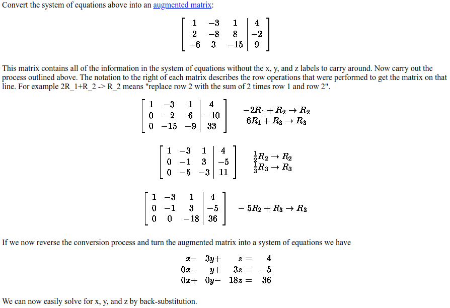
Gaussian elimination, also known as row reduction, is an algorithm in linear algebra for solving a system of linear equations. To perform row reduction on a matrix, one uses a sequence of elementary row operations to modify the matrix until the lower left-hand corner of the matrix is filled with zeros, as much as possible. There are three types of elementary row operations:
- Swapping two rows,
- Multiplying a row by a nonzero number,
- Adding a multiple of one row to another row.
Using these operations, a matrix can always be transformed into an upper triangular matrix, and in fact one that is in row echelon form. Once all of the leading coefficients (the leftmost nonzero entry in each row) are 1, and every column containing a leading coefficient has zeros elsewhere, the matrix is said to be in reduced row echelon form. This final form is unique; in other words, it is independent of the sequence of row operations used.
Vector spaces.
Image and kernel.
2. Analytic Geometry
- Norms. Discusses the notion of the length of vectors using the concept of a norm. A norm on a vector space V is a function:
$$||\cdot||:V \rightarrow \mathbb{R}, x \rightarrow ||x||$$
which assigns each vector $x$ its length $||x|| \in \mathbb{R}$, such that for all $\lambda \in \mathbb{R}$ and $x, y \in V$ the following hold:
- Absolutely homogeneous: $||\lambda x || = |\lambda|||x||$
- Triangle inequality: $||x + y|| \leq ||x|| + ||y||$
- Positive definite: $||x|| \geq 0$ and $||x|| = 0 \Leftrightarrow x = 0$
- Manhattan norm (L1 norm): on $\mathbb{R}^n$ is defined for $x \in \mathbb{R}^n$ as $$||x||1 := \sum{i=1}^{n}|x_i|$$
- Euclidean norm (L2 norm): on $\mathbb{R}^n$ is defined for $x \in \mathbb{R}^n$ as $$||x||2 := \sqrt{\sum{i=1}^{n}x_i^2}$$
- Inner product. A major purpose of inner products is to determine whether vectors are orthogonal to each other.
- Dot product is a particular type of inner product: $$x^Ty = \sum_{i=1}^{n}x_iy_i$$
- A symmetric matrix is a square matrix that is equal to its transpose.
- A symmetric $n \times n$ real matrix $M$ is said to be positive definite if the scalar $z^{T}Mz$ is strictly positive for every non-zero column vector $z$ of $n$ real numbers.
- We can compute lengths of vectors using the inner product.
- Algebraically, the dot product is the sum of the products of the corresponding entries of the two sequences of numbers. Geometrically, it is the product of the Euclidean magnitudes of the two vectors and the cosine of the angle between them.
- Two vectors $x$ and $y$ are orthogonal if and only if $<x, y> = 0$, and we write $x \perp y$.
- Inner product of functions. An inner product of two functions $u : \mathbb{R} \rightarrow \mathbb{R}$ and $v : \mathbb{R} \rightarrow \mathbb{R}$ can be defined as the definite integral: $$<u, v> := \int_{a}^{b} u(x)v(x) dx$$ If above integral evaluates to 0, then functions $u$ and $v$ are orthogonal. Furthermore, unlike inner products on finite-dimensional vectors, inner products on functions may diverge (have infinite value). As an example, for functions $u=sin(x)$ and $v=cos(x)$, since $\int_{a}^{b} u(x)v(x) dx$ evaluates to 0 in the limits of $a=-\pi$ and $b=\pi$, therefore $sin$ and $cos$ are orthogonal functions.
- We can project the original high-dimensional data onto a lower-dimensional feature space and work in this lower-dimensional space to learn more about the dataset and extract relevant patterns. PCA or autoencoders exploit this idea.
3. Matrix Decomposition
Determinant and trace. Determinants are only defined for square matrices $A \in \mathbb{R}^{n \times n}$. Determinant is a function that maps a matrix into a real number. It is calculated for $A \in \mathbb{R}^{2 \times 2}$ as: $$ det(A) = \begin{bmatrix} a_{11} & a_{12} \\ a_{21} & a_{22} \end{bmatrix} = a_{11}a_{22} - a_{12}a_{21} $$ The inverse of $A$ is $$ A^{-1} = \frac{1}{a_{11}a_{22} - a_{12}a_{21}} \begin{bmatrix} a_{11} & a_{12} \\ a_{21} & a_{22} \end{bmatrix} $$ Hence $A$ is invertible iff $$a_{11}a_{22} - a_{12}a_{21} \neq 0$$ This shows the relationship between determinants and the existence of inverse matrices. So for any square matrix $A \in \mathbb{R}^{n\times n}$ it holds that $A$ is invertible if and only if $det(A) \neq 0$.
For a triangular matrix, the determinant is the product of the diagonal elements.
Some properties of determinant is as follows:
- $det(AB) = det(A)det(B)$
- $det(A) = det(A^T)$
- $det(A^{-1}) = \frac{1}{det(A)}$
- Determinant is invariant to the choice of basis of a linear mapping.
- $det(\lambda A) = \lambda^n det(A)$
Eigenvalues and Eigenvectors. Let $A \in \mathbb{R}^{n \times n}$ be a square matrix. Then $\lambda \in \mathbb{R}$ is an eigenvalue of $A$ and $x \in \mathbb{R}^n\setminus{0}$ is the corresponding eigenvector of $A$ if $$Ax = \lambda x$$
- $\lambda$ is an eigenvalue of $A \in \mathbb{R}^{n \times n}$
- There exists an $x \in R^n\setminus{0}$ with $Ax = \lambda x$ or equivalently $x = 0$ can be solved non-trivially, i.e. $x \neq 0$.
- $det(A - \lambda I_n) = 0$.
The eigenvalue $\lambda$ tells whether the special vector $x$ is stretched or shrunk or reversed or left unchanged—when it is multiplied by $A$. We may find $\lambda = 2$ or 1/2 or 1 or -1. The eigenvalue could be zero! Then $Ax = 0x$ means that this eigenvector $x$ is in the nullspace. Geometrically, the eigenvector corresponding to a nonzero eigenvalue points in a direction that is stretched by the linear mapping. The eigenvalue is the factor by which it is stretched. If the eigenvalue is negative, the direction of the stretching is flipped.
- A matrix $A$ and its transpose $A^T$ possess the same eigenvalues, but not necessarily the same eigenvectors.
- Symmetric, positive definite matrices always have positive, real eigenvalues.
- Similar matrices possess the same eigenvalues. Therefore, a linear mapping $\Phi$ has eigenvalues that are independent of the choice of basis of its transformation matrix. This makes eigenvalues, together with the determinant and the trace, key characteristic parameters of a linear mapping as they are all invariant under basis change.
Given a matrix $A \in R^{m \times n}$, we can always obtain a symmetric, positive semidefinite matrix $S \in R^{n \times n}$ by defining $$S := A^TA$$ The determinant of a matrix $A \in R^{n \times n}$ is the product of its eigenvalues, i.e., $$det(A) = \prod_{i=1}^{n} \lambda_i$$ where $\lambda_i$ are (possibly repeated) eigenvalues of $A$.
4. Vector Calculus
- For $h > 0$ the derivative of $f$ at $x$ is defined as the limit: $$\frac{df}{dx} := \lim_{h \rightarrow 0} \frac{f(x+h) - f(x}{h}$$
- The derivative of $f$ points in the direction of steepest ascent of $f$.
- Taylor series is a representation of a function $f$ as an infinite sum of terms. These terms are determined using derivatives of $f$ evaluated at $x_0$. The Taylor polynomial of degree $n$ of $f : \mathbb{R} \rightarrow \mathbb{R}$ at $x_0$ is defined as $$T_n(x) := \sum_{k=0}^{n}\frac{f^{(k)}(x_0)}{k!} (x-x_0)^k$$ where $f^{(k)}(x_0)$ is the $k$th derivative of $f$ at $x_0$ and $\frac{f^{(k)}(x_0)}{k!}$ are the coefficients of the polynomial.
- Differentiation rules:
- $(f(x)g(x))’ = f’(x)g(x) + f(x)g’(x)$
- $(\frac{f(x)}{g(x)})’ = \frac{f’(x)g(x) - f(x)g’(x)}{(g(x))^2}$
- $(f(x) + g(x))’ = f’(x) + g’(x)$
- $(g(f(x)))’ = (gof)’(x) = g’(f(x))f’(x)$
- The generalization of the derivative to functions of several variables is the gradient.
- Chain rule: $$\frac{d}{dx}(g(f(x)) = \frac{dg}{df}\frac{df}{dx}$$
- The collection of all first-order partial derivatives of a vector-valued function $f: \mathbb{R}^n \rightarrow \mathbb{R}^m$ is called the Jacobian.
- In deep learning, we have $$y = (f_k o f_{k-1} o … o f_1)(x) = f_k(f_{k-1}(…(f_1(x))…))$$ where $x$ are the inputs, $y$ are the observations, and every function $f_i, i=1,…,k$, possesses its own parameters.
- The Hessian is the collection of all second-order partial derivatives. As an example $$ H= \begin{bmatrix} \frac{d^2f}{dx^2} & \frac{d^2f}{dxdy} \\ \frac{d^2f}{dxdy} & \frac{d^2f}{dy^2} \end{bmatrix} $$ The Hessian measures the curvature of the function locally around $(x, y)$.
5. Probability and Distributions
Probability space:
- The sample space $\Omega$: The sample space is the set of all possible outcomes of the experiment, usually denoted by $\Omega$.
- The event space $A$: The event space is the space of potential results of the experiment. A subset $A$ of the sample space $\Omega$ is in the event space $A$ if at the end of the experiment we can observe whether a particular outcome $\omega \in \Omega$ is in $A$.
- The probability $P$: With each event $A \in A$, we associate a number $P(A)$ that measures the probability or degree of belief that the event will occur.
In machine learning, we often avoid explicitly referring to the probability space, but instead refer to probabilities on quantities of interest, which we denote by $T$. We refer to $T$ as target space. Association or mapping from $\Omega$ to $T$ is called a random variable.
Probability density function (PDF): A function $f: \mathbb{R}^D \rightarrow \mathbb{R}$ is called a PDF if:
- $\forall x \in \mathbb{R}^D : f(x) \geqslant 0$
- Its integral exists and $$\int_{\mathbb{R}^D} f(x)dx = 1$$
In a more precise sense, the PDF is used to specify the probability of the random variable falling within a particular range of values, as opposed to taking on any one value. For probability mass functions (PMF) of discrete random variables, the integral is replaced with a sum. We associate a random variable $X$ with this function $f$ by $$P(a \leqslant X \leqslant b) = \int_{a}^{b} f(x)dx$$ where $a, b \in \mathbb{R}$ and $x \in \mathbb{R}$ are outcomes of the continuous random variable $X$. In contrast to discrete random variables, the probability of a continuous random variable $X$ taking a particular value $P (X = x)$ is zero.
Sum rule (marginalization property): $$ p(x) = \begin{cases} \sum_{y \in Y} p(x,y) \qquad \text{if y is discrete}\\ \int_{y} p(x,y)dy \qquad \text{if y is continuous} \end{cases} $$
Product rule: $$p(x,y)=p(y|x)p(x)$$ Bayes’ rule: $$p(x|y) = \frac{p(y|x)p(x)}{p(y)}$$ where $p(x|y)$ is posterior, $p(y|x)$ is likelihood, $p(x)$ is prior, and $p(y)$ is evidence. Bayes’ rule allows us to invert the relationship between $x$ and $y$ given by the likelihood.
Expected value of a function $g : \mathbb{R} \rightarrow \mathbb{R}$ of a univariate continuous random variable $X \sim p(x)$ is given by $$E_X [g(x)] = \int_{X} g(x)p(x)dx$$
Mean of a random variable $X$ with states $x \in \mathbb{R}^D$ is an average and is defined as $$ E_X[x] = \begin{bmatrix} E_{X_1} [x_1] \\ .\\ .\\ .\\ E_{X_D} [x_D] \end{bmatrix} \in \mathbb{R}^D $$ where $$ E_{X_d} [x_d] := \begin{cases} \sum_{x_i \in X} x_i p(x_d=x_i) \qquad \text{if X is a discrete random variable}\\ \int_{X} x_d p(x_d) dx_d \qquad \text{if X is a continuous random variable} \end{cases} $$
Two random variables are independent iff $$p(x,y) = p(x)p(y)$$ If $x,y$ are independent, then:
- $p(x|y) = p(x)$ and $p(y|x) = p(y)$
- $p(x|y,z) = p(x|z)$
Gaussian distribution. For a univariate random variable, the Gaussian distribution has a density that is given by $$p(x| \mu, \sigma^2) = \frac{1}{\sqrt{2 \pi \sigma^2}} exp (-\frac{(x-\mu)^2}{2 \sigma^2})$$ The univariate Gaussian distribution (or “normal distribution,” or “bell curve”) is the distribution you get when you do the same thing over and over again and average the results.
Bernoulli distribution is a distribution for a single binary random variable $X$ with state $x \in {0, 1}$. It is governed by a single continuous parameter $\mu \in [0, 1]$ that represents the probability of $X = 1$. The Bernoulli distribution $Ber(\mu)$ is defined as $$p(x|\mu) = \mu^x (1-\mu)^{1-x}, \qquad x \in {0, 1}$$ $$E[x] = \mu$$ $$V[x] = \mu(1-\mu)$$ where $E[x]$ and $V[x]$ are the mean and variance of the binary random variable $X$.
Binomial distribution is a generalization of the Bernoulli distribution to a distribution over integers. In particular, the Binomial can be used to describe the probability of observing $m$ occurrences of $X = 1$ in a set of $N$ samples from a Bernoulli distribution where $p(X = 1) = \mu \in [0, 1]$. The Binomial distribution $Bin(N, \mu)$ is defined as $$p(m|N,\mu) = {{N}\choose{m}} \mu^m (1-\mu)^{N-m}$$ $$E[m] = N\mu$$ $$V[m] = N\mu (1-\mu)$$ where $E[x]$ and $V[x]$ are the mean and variance of $m$, respectively. An example where the Binomial could be used is if we want to describe the probability of observing $m$ heads in $N$ coin-flip experiments if the probability for observing head in a single experiment is $\mu$.
Beta distribution is a distribution over a continuous random variable $\mu \in [0, 1]$, which is often used to represent the probability for some binary event (e.g., the parameter governing the Bernoulli distribution). The Beta distribution $Beta(\alpha, \beta)$ itself is governed by two parameters $\alpha > 0, \beta > 0$ and is defined as $$p(\mu | \alpha, \beta) = \frac{\Gamma(\alpha + \beta)}{\Gamma(\alpha)\Gamma(\beta)}\mu^{\alpha -1}(1-\mu)^{\beta -1}$$ $$E[\mu] = \frac{\alpha}{\alpha + \beta}$$ $$V[\mu] = \frac{\alpha\beta}{(\alpha+\beta)^2(\alpha + \beta +1)}$$ where $\Gamma(.)$ is the Gamma function defined as $$\Gamma(t) := \int_{0}^{\infty} x^{t-1} exp(-x)dx \qquad t > 0$$ $$\Gamma(t+1) = t\Gamma(t)$$ Intuitively, $\alpha$ moves probability mass toward 1, whereas $\beta$ moves probability mass toward 0.
6. Continuous Optimization
Convex functions do not exhibit tricky dependency on the starting point of the optimization algorithm. For convex functions, all local minimums are global minimum. It turns out that many machine learning objective functions are designed such that they are convex.
For a differentiable function, if $$x_1 = x_0 - \gamma ((\nabla f)(x_0))^T$$ for a small step-site $\gamma \geq 0$, then $f(x_1) \leq f(x_0)$. The sequence $f(x_0) \geq f(x_1) \geq …$ converges to a local minimum.
Choosing a good step-size is important in gradient descent. If the step-size is too small, gradient descent can be slow. If the step-size is chosen too large, gradient descent can overshoot, fail to converge, or even diverge. Adaptive gradient methods rescale the step-size at each iteration, depending on local properties of the function. There are two simple heuristics:
- When the function value increases after a gradient step, the step-size was too large. Undo the step and decrease the step-size.
- When the function value decreases the step could have been larger. Try to increase the step-size.
Gradient descent with momentum is a method that introduces an additional term to remember what happened in the previous iteration. This memory dampens oscillations and smoothes out the gradient updates. The momentum-based method remembers the update $\Delta x_i$ at each iteration $i$ and determines the next update as a linear combination of the current and previous gradients $$x_{i+1} = x_i - \gamma_i((\nabla f)(x_i))^T + \alpha \Delta x_i$$ $$\Delta x_i = x_i - x_{i-1}$$ where $\alpha \in [0,1]$.
Computing the gradient can be very time consuming. However, often it is possible to find a “cheap” approximation of the gradient. Approximating the gradient is still useful as long as it points in roughly the same direction as the true gradient. Stochastic gradient descent (often shortened as SGD) is a stochastic approximation of the gradient descent method for minimizing an objective function that is written as a sum of differentiable functions. The word stochastic here refers to the fact that we acknowledge that we do not know the gradient precisely, but instead only know a noisy approximation to it.
Given $n=1,…,N$ data points, objective function can be defined as $$L(\theta) = \sum_{n=1}^{N} L_n(\theta)$$ where $\theta$ is the set of parameters of the network. By updating the vector of parameters according to $$\theta_{i+1} = \theta_i - \gamma_i(\nabla L(\theta_i))^T = \theta_i - \gamma_i \sum_{n=1}^{N}(\nabla L_n(\theta_i))^T$$ When the training set is enormous and/or no simple formulas exist, evaluating the sums of gradients becomes very expensive. Considering the term $\sum_{n=1}^{N}(\nabla L_n(\theta_i))^T$, we can reduce the amount of computation by taking a sum over a smaller set of $L_n$. In contrast to batch gradient descent, which uses all $L_n$ for $n = 1, …, N$, we randomly choose a subset of $L_n$ for mini-batch gradient descent. The key insight about why taking a subset of data is sensible is to realize that for gradient descent to converge, we only require that the gradient is an unbiased estimate of the true gradient.
Constrained Optimization and Lagrange Multipliers. What if there are additional constraints? That is, for real-valued functions $g_i: \mathbb{R}^D \rightarrow \mathbb{R}$ for $i=1,…,m$, we consider the constrained optimization problem $$\min_{x} f(x)$$ subject to $g_i(x) \leq 0$ for all $i=1,…,m$
One obvious, but not very practical, way of converting the constrained problem into an unconstrained one is to use an indicator function $$J(x) = f(x) + \sum_{i=1}^{m}1(g_i(x))$$ where $1(z)$ is an infinite step function $$ 1(z) = \begin{cases} 0 \qquad z \leq 0\\ \infty \qquad otherwise \end{cases}$$ This gives infinite penalty if the constraint is not satisfied, and hence would provide the same solution. However, this infinite step function is equally difficult to optimize. We can overcome this difficulty by introducing Lagrange multipliers. The idea of Lagrange multipliers is to replace the step function with a linear function. We do this by introducing the Lagrange multipliers $\lambda_i \geq 0$ corresponding to each inequality constraint respectively so that $$L(x, \lambda) = f(x) + \sum_{i=1}^{m}\lambda_i g_i(x) = f(x) + \lambda^Tg(x)$$ In general, duality in optimization is the idea of converting an optimization problem in one set of variables $x$ (called the primal variables), into another optimization problem in a different set of variables $\lambda$ (called the dual variables). The main problem is $$\min_{x} f(x)$$ subject to $g_i(x) \leq 0$ for all $i=1,…,m$ and its associated Lagrangian dual problem is given by $$\max_{\lambda \in \mathbb{R}^m} D(\lambda)$$ subject to $\lambda \geq 0$ where $\lambda$ are the dual variables and $D(\lambda)=min_{x\in \mathbb{R}^d} L(x, \lambda)$.
Convex optimization. A set $C$ is a convex set if for any $x, y \in C$ and for any scalar $\theta$ with $0 \leq \theta \leq 1$, we have $$\theta x + (1-\theta)y \in C$$ Convex sets are sets such that a straight line connecting any two elements of the set lie inside the set. Convex functions are functions such that a straight line between any two points of the function lie above the function.
Let function $f:\mathbb{R}^D \rightarrow \mathbb{R}$ be a function whose domain is a convex set. The function $f$ is a convex function if for all $x, y$ in the domain of $f$, and for any scalar $\theta$ with $0 \leq \theta \leq 1$, we have $$f(\theta x + (1-\theta)y) \leq \theta f(x) + (1-\theta)f(y)$$ A concave function is the negative of a convex function.
7. When Models Meet Data
- The distinction between parameters and hyperparameters is somewhat arbitrary, and is mostly driven by the distinction between what can be numerically optimized versus what needs to use search techniques. Another way to consider the distinction is to consider parameters as the explicit parameters of a probabilistic model, and to consider hyperparameters (higher-level parameters) as parameters that control the distribution of these explicit parameters.
- The set of examples $(x_1, y_1), … ,(x_N, y_N)$ is independent and identically distributed. The word independent means that two data points $(x_i, y_i)$ and $(x_j, y_j)$ do not statistically depend on each other, meaning that the empirical mean is a good estimate of the population mean. This implies that we can use the empirical mean of the loss on the training data.
- In principle, the design of the loss function for empirical risk minimization should correspond directly to the performance measure specified by the machine learning task.
- The idea behind maximum likelihood estimation (MLE) is to define a function of the parameters that enables us to find a model that fits the data well. For data represented by a random variable $x$ and for a family of probability densities $p(x | \theta)$ parametrized by $\theta$, the negative log-likelihood is given by $$L_x(\theta) = -log p(x|\theta)$$
- If we have prior knowledge about the distribution of the parameters $\theta$, we can multiply an additional term to the likelihood. This additional term is a prior probability distribution on parameters $p(\theta)$. Bayes’ theorem allows us to compute a posterior distribution $p(\theta, x)$ (the more specific knowledge) on the parameters $\theta$ from general prior statements (prior distribution) $p(\theta)$ and the function $p(x, \theta)$ that prior links the parameters $\theta$ and the observed data $x$ (called the likelihood): $$p(\theta|x) = \frac{p(x|\theta)p(\theta)}{p(x)}$$ Recall that we are interested in finding the parameter $\theta$ that maximizes the posterior. Since the distribution $p(x)$ does not depend on $\theta$, we can ignore the value of the denominator for the optimization and obtain $$p(\theta|x) \propto p(x|\theta)p(\theta)$$
8. Linear Regression (Curve Fitting)
- In regression, we aim to find a function $f$ that maps inputs $x \in \mathbb{R}^D$ to corresponding function values $f(x) \in \mathbb{R}$. We assume we are given a set of training inputs $x_n$ and corresponding noisy observations $y_n = f(x_n)+\epsilon$, where $\epsilon$ is an i.i.d. random variable that describes measurement/observation noise and potentially unmodeled processes.
- A widely used approach to finding the desired parameters $\theta_{ML}$ is maximum likelihood estimation. Intuitively, maximizing the likelihood means maximizing the predictive distribution of the training data given the model parameters. The likelihood $p(y | x, \theta)$ is not a probability distribution in $\theta$: It is simply a function of the parameters $\theta$ but does not integrate to 1 (i.e.,it is unnormalized), and may not even be integrable with respect to $\theta$. To find the desired parameters $\theta_{ML}$ that maximize the likelihood, we typically perform gradient ascent (or gradient descent on the negative likelihood).
- linear regression offers us a way to fit nonlinear functions within the linear regression framework: Since “linear regression” only refers to “linear in the parameters”, we can perform an arbitrary nonlinear transformation $\phi(x)$ of the inputs $x$ and then linearly combine the components of this transformation.
9. Dimensionality Reduction with Principal Component Analysis
- In PCA, we are interested in finding projections $\tilde{x}_n$ of data points $x_n$ that are as similar to the original data points as possible, but which have a significantly lower intrinsic dimensionality.
- The variance of the data projected onto a one-dimensional subspace equals the eigenvalue that is associated with the basis vector b1 that spans this subspace. Therefore, to maximize the variance of the low-dimensional code, we choose the basis vector associated with the largest eigenvalue of the data covariance matrix. This eigenvector is called the first principal component.
- In the following, we will go through the individual steps of PCA using a running example. We are given a two-dimensional dataset, and we want to use PCA to project it onto a one-dimensional subspace.
- Mean subtraction: We start by centering the data by computing the mean $\mu$ of the dataset and subtracting it from every single data point. This ensures that the dataset has mean 0. Mean subtraction is not strictly necessary but reduces the risk of numerical problems.
- Standardization: Divide the data points by the standard deviation $\sigma_d$ of the dataset for every dimension $d = 1,…,D$. Now the data is unit free, and it has variance 1 along each axis. This step completes the standardization of the data.
- Eigendecomposition of the covariance matrix: Compute the data covariance matrix and its eigenvalues and corresponding eigenvectors. Since the covariance matrix is symmetric, the spectral theorem states that we can find an ONB of eigenvectors.
- Projection: We can project any data point $x_* \in \mathbb{R}^D$ onto the principal subspace: To get this right, we need to standardize $x_*$ using the mean $\mu_d$ and standard deviation $\sigma_d$ of the training data in the $d$th dimension, respectively.
10. Classification with Support Vector Machines
- The maximum likelihood view proposes a model based on a probabilistic view of the data distribution, from which an optimization problem is derived. In contrast, the SVM view starts by designing a particular function that is to be optimized during training, based on geometric intuitions.
- Given two examples represented as vectors $x_i$ and $x_j$, one way to compute the similarity between them is using an inner product $<x_i, x_j>$. Recall that inner products are closely related to the angle between two vectors. The value of the inner product between two vectors depends on the length (norm) of each vector. Furthermore, inner products allow us to rigorously define geometric concepts such as orthogonality and projections.
- The concept of the margin turns out to be highly pervasive in machine learning.
- In the case where data is not linearly separable, we may wish to allow some examples to fall within the margin region, or even to be on the wrong side of the hyperplane. The model that allows for some classification errors is called the soft margin SVM.
- The function of kernel is to take data as input and transform it into the required form. The kernel function is what is applied on each data instance to map the original non-linear observations into a higher-dimensional space in which they become separable.
{% endraw %}